In the previous chapter, I introduced the core indexes within SQL Server, both rowstore and columnstore, clustered and nonclustered. This chapter takes that information and adds additional functionality to those indexes. I’ll also introduce some new indexes in this chapter. There are a number of index settings that affect their behavior which we’ll also discuss.
Covering indexes
Index intersection
Index joins
Filtered indexes
Indexed views
Index characteristics
Special index types
Covering Indexes
A covering index is a nonclustered index that contains all the columns required to satisfy a query without going to the heap or the clustered index. We’ve already had several covering indexes in examples throughout the book.
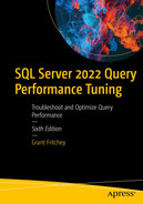
A query that does not have a covering index
A diagram begins on the right with a non-clustered index seek and clustered key lookup with values of, 13% cost, 0.006 seconds, 8 of 8, and 87%, 0.007 seconds, 8 of 8, given, respectively.
Execution plan for a query without a covering index
Recreating the IX_Address_StateProvinceID index
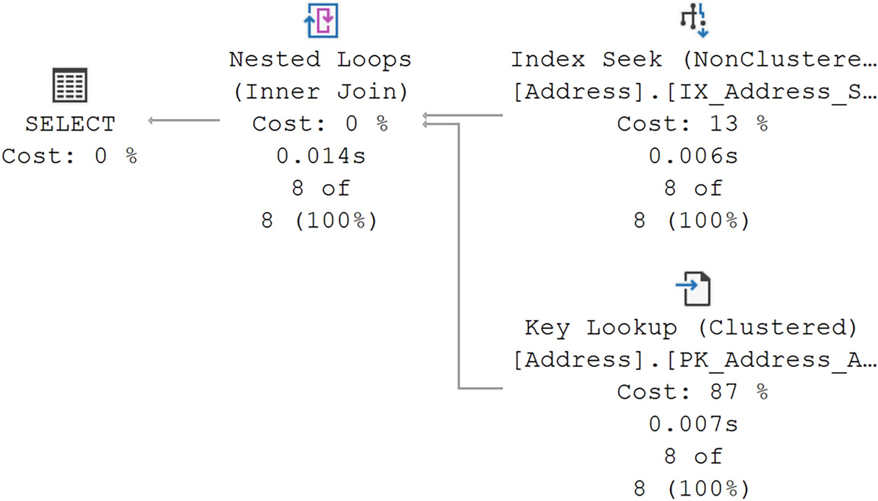
A diagram begins on the right with a non clustered index seek with values of 100% cost, 0.000 seconds, and 8 of 8, given, and select on the left with 0% cost.
Execution plan for the query with a covering index
Performance was more than cut in half, and the reads went from 19 to 2. You can see the results in the execution plan where only our nonclustered index was referenced. Clearly, a covering index can be a useful mechanism for increasing query performance. Modifying the key of the index would have done the same thing, but then the index would be structurally different. Using the INCLUDE operator worked because we didn’t need that column to be used in a WHERE, JOIN, or HAVING clause. If that was the case, you’d then be better off modifying the key.
Reverting the index to its previous shape
A Pseudoclustered Index
A covering index physically organizes the data in the key columns in a sequential order, in the order of the keys. Any data included at the leaf level is then ordered by the key column(s) in the same way. That means, for a query this index satisfies as covering, it becomes effectively the same as a clustered index. In some cases, you’ll see superior performance from a covering index, even when the data is being ordered, over a clustered index because the covering, nonclustered, index is generally smaller, with only a subset of the columns of the clustered index.
Conversely, you can make a nonclustering index effectively a full clustered index by adding all the columns through INCLUDE. However, this adds the possibility of considerable overhead since any change to any column now results in updates to the clustered index and the nonclustered index.
Recommendations
A common, and old, admonition when it comes to writing queries is to only move the data you need. This is why people will frequently advocate against using SELECT *. The same is true of trying to make an index into a covering index. Be judicious in the columns that you add, either to the key or through the INCLUDE operation. If you do add columns to the key of the index, you are making that index wider, allowing for fewer rows per page, which could also hurt performance. All of this is absolutely a balancing act and why it’s so important to set up testing for your systems to ensure you know how these changes are going to affect other queries.
Index Intersection
When there are multiple indexes on a table, SQL Server can use more than one index to satisfy a query. It will use a set of data from each index and then combine them for a result. This combination of indexes is called index intersection. While it sounds like a great thing, it’s actually pretty rare to see it in action. You can’t count on it as a regular occurrence.
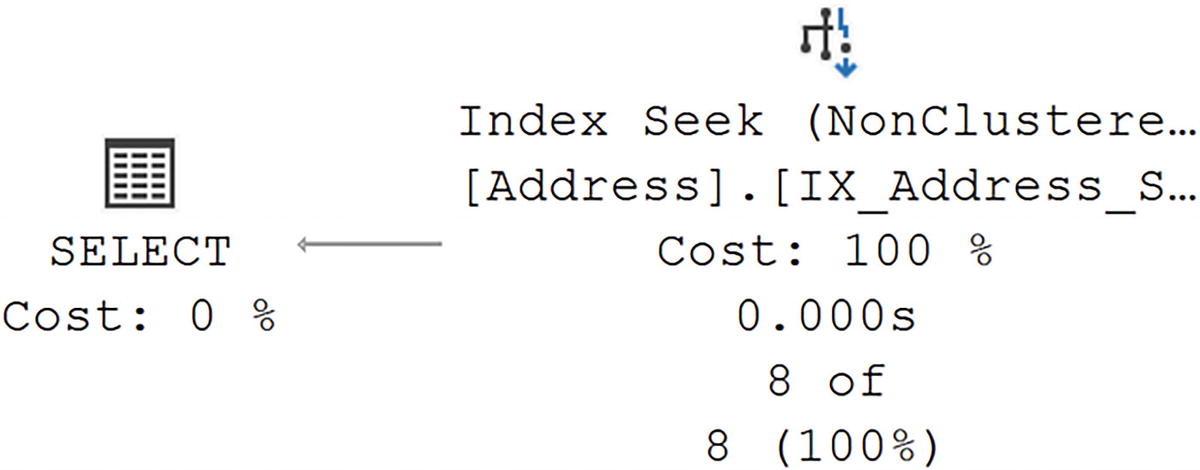
A query performing a Clustered Index Scan
A diagram begins on the right with a clustered index scan with values of 100% cost, 0.002 seconds, and 36 of 95, given, and select on the left with 0% cost.
No indexes help the query, so a scan ensues
Adding an index in the hopes of index intersection
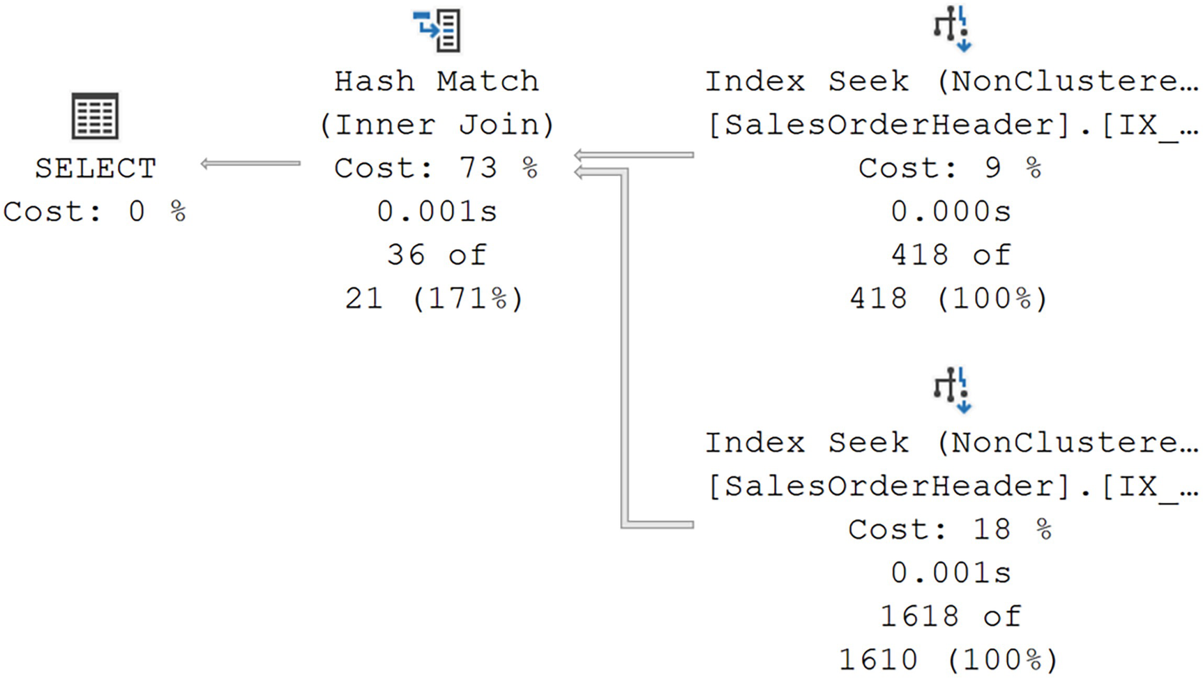
A diagram begins on the right with 2 non clustered index seeks with values of, 9% cost, 0.000 seconds, 418 of 418, and 18%, 0.001 seconds,1618 of 1610, given, respectively. Then to hash match, inner join with values of 73% cost, 0.001 seconds, and 36 of 21, and select at 0%.
An index intersection
We’ve successfully arrived at an index intersection. The key point here is the Hash Match join. If we saw either a Nested Loops or Merge, that would be an index join (covered in the next section), which is extremely similar to index intersection, but not exactly the same.
In an index intersection, the optimizer has assumed it can put together a match, but it doesn’t have a guaranteed mechanism to ensure the match. If it did, you’d see the other join types. The optimizer has chosen to build a temporary table (the hash table), and the probe against that has to find the combined data. So it seeks 418 rows from one index and 1,618 from the other and then combines them into 36 matching rows (per the values in the execution plan with runtime metrics).
The performance went from 4ms to 2.8ms, which isn’t huge. However, the reads went from 689 to 10. That’s the difference between index seeks and an index scan, even if you have to then process a join to get to the result set.
Creating a compound key on the test index
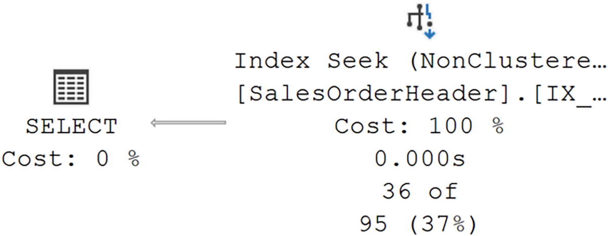
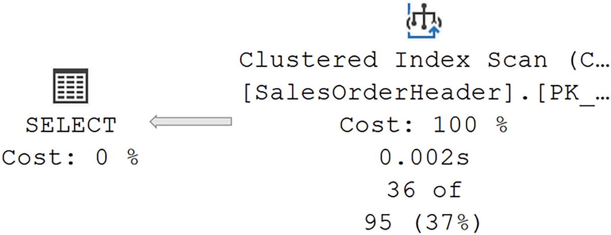
A diagram begins on the right with a non clustered index seek with values of 100% cost, 0.000 seconds, and 36 of 95, given, and select on the left, with 0% cost.
Replacing the index intersection
Now we see a radical improvement in performance, going from 2.8ms to 252mcs and from 6 reads to 2. Creating a compound key, while it did change the index structure and make the index wider, resulted in an even more serious performance improvement.
Reordering the columns in one of the existing indexes would have a negative impact on other queries.
Some of the columns required to make a covering index are not a part of the existing indexes.
If you are limited in the changes you can make to an index, sometimes, just adding another nonclustered index might be a good solution if it results in index intersection, or, as we’ll see in a second, an index join.
Removing the test index
Index Joins
A query that will perform an index join
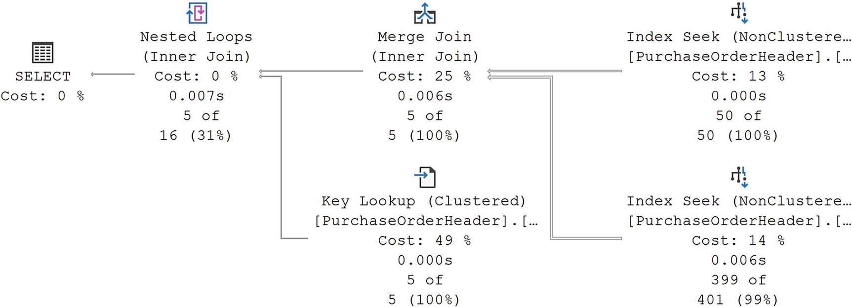
A diagram begins on the right with 2 non clustered index seeks with values of, 13% cost, 0.000 seconds, 50 of 50, and 14%, 0.006 seconds, 399 of 401, given, respectively. On the left are merge join and clustered key lookup with costs of 25% and 49%, respectively.
An index join
There are a couple of points to make here. First, you see the two indexes being used to seek for the appropriate data in the filter criteria. One is from the index on EmployeeID, and one is from the index on VendorID. They are then using a Merge Join to combine the two data sets.
Second, note the Key Lookup operation. Because I included the RevisionNumber column, the join between the two indexes was not covering. That means it had to go to the clustered index to retrieve the rest of the data. In most circumstances, you won’t see this with an index intersection. The combined indexes have to be covering. However, with an index join, you can see lookups.
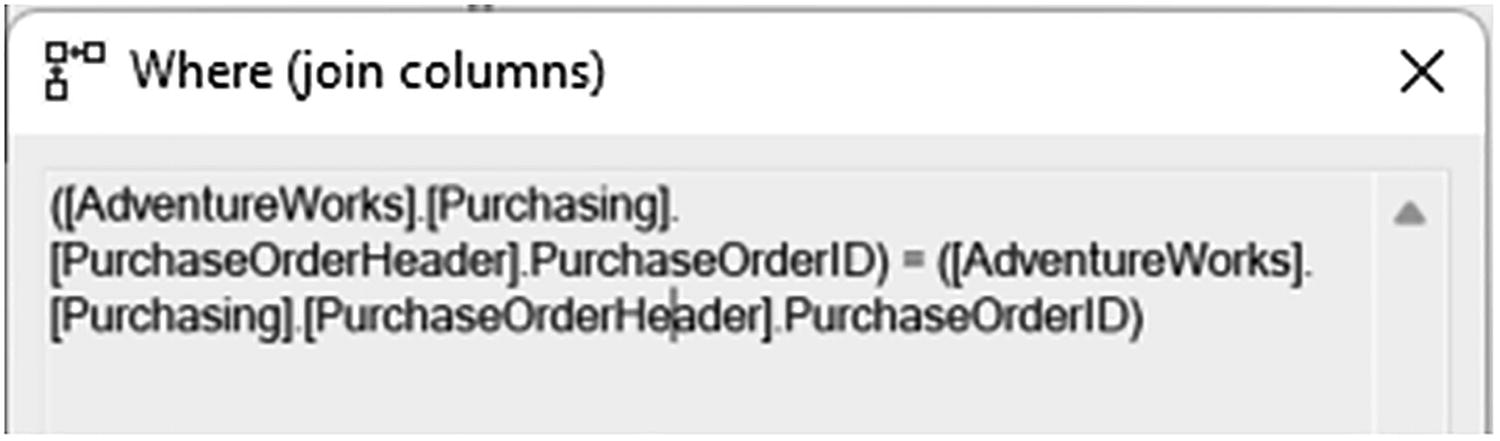
A window of the merge join operator has 3 lines of text. The first line reads as open parenthesis, open square bracket, Adventure Works, close square bracket, period, open square bracket, Purchasing, close square bracket, period.
Join criteria in the Where (join columns) property
As was shown in the previous section, sometimes, wider indexes perform better. Sometimes, you may find that index intersection and index join allow you to use narrower indexes. Testing and validation are always going to be necessary to know what’s going to work best for a given query, within a given system.
Filtered Indexes
A filtered index is a nonclustered rowstore index that uses a filter, simply a WHERE clause, to create a more selective index. For example, a column with a large number of NULL values may be stored as a sparse column to reduce the overhead of those NULL values. Adding an index that eliminates NULLs could be useful.
A query to retrieve purchase order numbers
An index to improve query performance
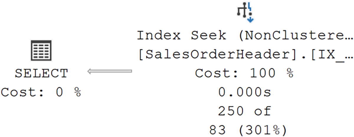
A diagram begins on the right with a non clustered index seek with values of 100% cost, 0.000 seconds, and 250 of 83, given, and select on the left, with 0% cost.
The scan is gone, and an index seek is operating
Eliminating the NULL values from the index
I recognize that’s not a major performance enhancement. However, it’s better. Imagine this query is called thousands of times a minute. Reducing its time and resource use constitutes a win.
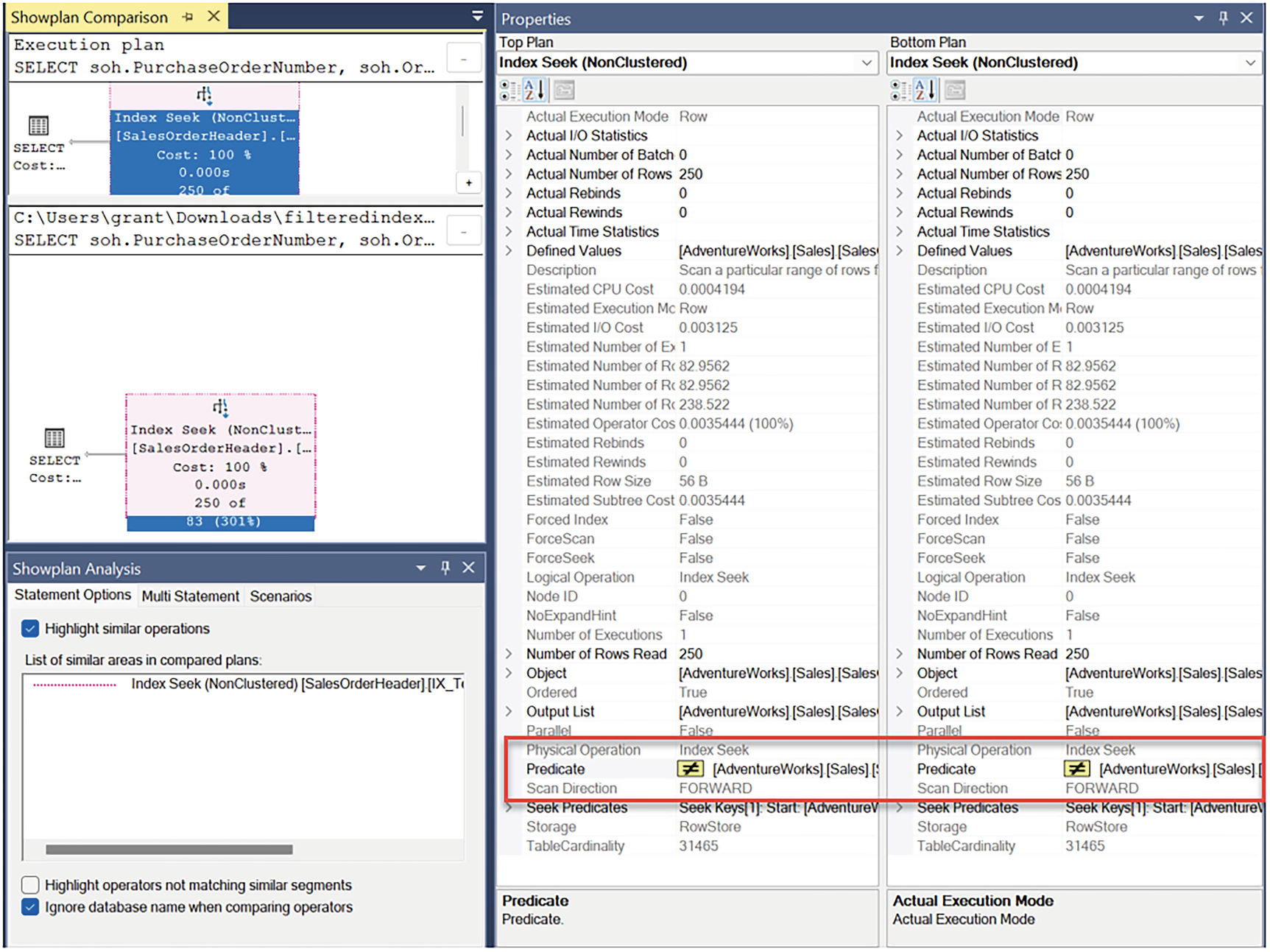
A window has an execution plan pane on the upper half of the left panel and a show plan analysis pane below it, with the text, highlight similar options, ticked. On the right are the top and bottom plan panes where the entries are boxed,
Comparison between two nearly identical execution plans
You’ll notice that almost every single property in both Index Seek operators is identical. However, the one difference is highlighted. It’s the Predicate. The simplification process within the query optimizer removed the IS NOT NULL from the query since the index eliminates NULL values.
While filtered indexes can improve performance, they are not without cost. You might see issues where parameterized queries don’t perfectly match the WHERE clause in the index, therefore preventing its use. Statistics are not updated on the filtering criteria, but rather on the entire table, just like a regular index. Testing on your own system to see where, and when, this helps performance is a must.
The most frequent purpose for using filtered index is the example we just saw, the elimination of NULL values. You can also isolate frequently accessed sets of data with a filtered index so that queries against that data perform faster. You can use the WHERE clause to filter data in ways that are similar to creating indexed views (covered in the next section) without the extensive data maintenance headaches associated with indexed views. Following the example shown previously and making the nonclustered, filtered, index into a covering index further enhance performance.
On: ANSI_NULLS, ANSI_PADDING, ANSI_WARNINGS, ARITHABORT, CONCAT_NULL_YIELDS_NULL, and QUOTED_IDENTIFIER
Off: NUMERIC_ROUNDABORT
Removing the test index
Indexed Views
A view in SQL Server does not store any data. A view is simply a SELECT statement, stored within an object called a view. That view does act as if it were a table, but it’s just a query. You define a view using the CREATE VIEW command. Once created, it can be used like a table.
You can also take a view and perform an action called materialization. You’re basically creating a new clustered index, based on the query that defines the view. This is called an indexed view or a materialized view. When you create a materialized view, the data is actually persisted to disk and stored within the database, at which point, it is, to all intents and purposes, effectively the same as a table. You can even create nonclustered indexes on the indexed view.
Benefit
Aggregations can be precomputed and stored in the indexed view to minimize expensive computations during query execution.
Tables can be pre-joined, and the resulting data set is materialized.
Combinations of joins or aggregations can also be materialized.
Overhead
Any change in the base tables has to be reflected in the indexed view by executing the view’s SELECT statement.
Any changes to a base table on which an indexed view is defined may initiate one or more changes in the nonclustered indexes on the indexed view. The clustered index will also have to be changed if the clustering key is updated.
The indexed view adds to the ongoing maintenance overhead of the database, along with the statistics that also must be maintained.
Additional storage is required.
Whatever keys define the indexed view, it must be a unique index.
Nonclustered indexes on an indexed view can be created only after the unique clustered index is created.
The view definition must be deterministic—that is, it is able to return only one possible result for a given query (a list of deterministic and nondeterministic functions is available in the SQL Server documentation).
The indexed view must reference only base tables in the same database, not other views.
The indexed view must be schema bound to the tables referred to in the view to prevent modifications of the table (frequently a major problem).
There are several restrictions on the syntax of the view definition (a complete list is provided in the SQL Server documentation).
- The list of SET options that must be set is as follows:
On: ARITHABORT, CONCAT_NULL_YIELDS_NULL, QUOTED_IDENTIFIER, ANSI_NULLS, ANSI_PADDING, and ANSI_WARNING
Off: NUMERIC_ROUNDABORT
Usage Scenarios
Dedicated reporting and analysis systems generally benefit the most from indexed views. OLTP systems with frequent writes may not be able to take advantage of indexed views because of the increased maintenance overhead associated with updating both the underlying tables and the view itself, all within a single transaction. The net performance improvement provided by an indexed view is the difference between the total query execution savings and the cost of storing and maintaining the view. Careful testing here is a must.
If you are using the Enterprise edition of SQL Server (or the Developer edition), an indexed view need not be referenced in the query for the query optimizer to use it during query execution. This allows existing applications to benefit from the newly created indexed views without changing those applications. Otherwise, you would need to directly reference the view within your T-SQL code. The query optimizer considers indexed views only for queries with nontrivial cost. You may also find that a columnstore index will work better for you than indexed views, especially when you’re running aggregation or analysis queries.
Analysis style queries
Creating an indexed view
As I mentioned earlier, some functions, such as AVG, are disallowed since it’s nondeterministic (again, the complete list is in the SQL Server documentation). If aggregates are included in the view, you must include COUNT_BIG by default.
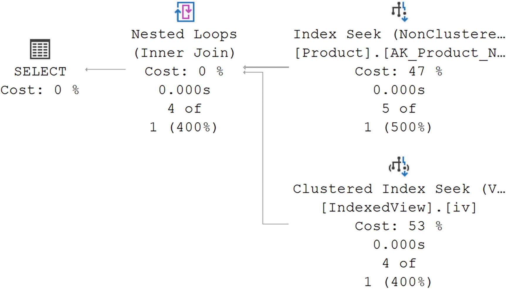
A diagram begins on the right with a non-clustered index seek and clustered index seek with values of, 47% cost, 0.000 seconds, 5 of 1, and 53%, 0.000 seconds, 4 of 1, given, respectively. Then to the nested loops, inner join with values of 0% cost, 0.000 seconds, and 4 of 1.
The use of an indexed view in a query
The optimizer can tell that the indexed view can satisfy the needs of the query, so it just uses that instead of the tables.
Removing the indexed view
Index Compression
Using compression on an index means using algorithms to reduce the amount of space taken up by data, thereby putting more data on a given page. More data on a page means fewer pages need to be read from disk. Fewer reads mean better performance. You also get the compressed pages in memory, so you’re reducing memory use as well. You will see added overhead on the CPU since compression and decompression will be going through calculations. This overhead means that this won’t be a viable solution for all indexes.
By default, indexes are not compressed. You have to call for compression on your indexes. There are two different kinds of index compression: row- and page-level compression. Row-level compression identifies the columns that can be compressed (for details, see the SQL Server documentation) and then compresses the data in that column. It does this on a row-by-row basis. Page-level compression actually does row-level compression and then additional compression on top to reduce storage size for the non-row elements stored on a page. Non-leaf pages in an index receive no compression under the page type.
Creating a noncompressed index
Creating compressed indexes
Getting a count of pages and compressed pages
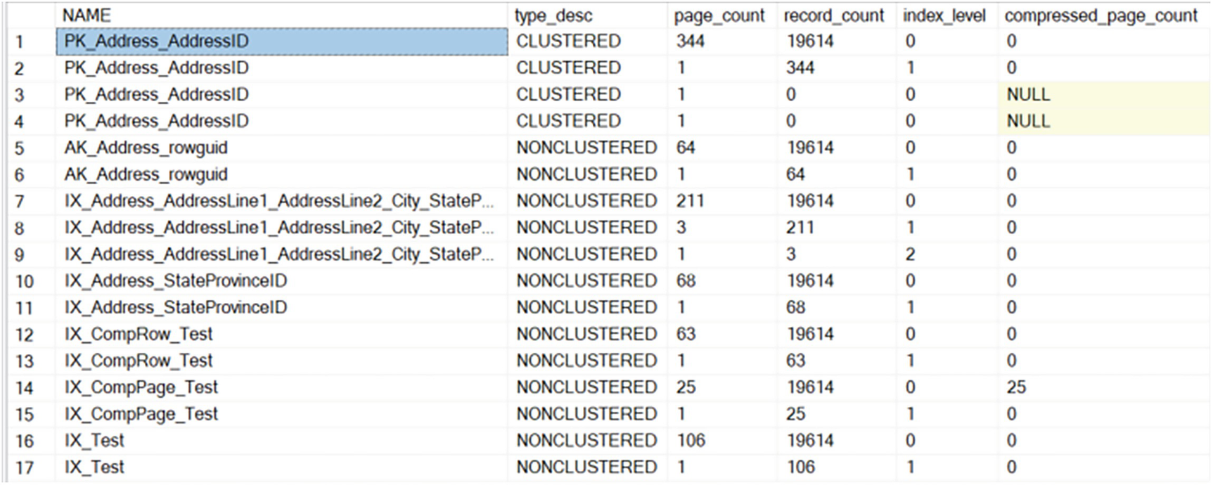
A table has 6 columns and 17 rows, with column headers, name, type description, page count, record count, index level, and compressed page count. The first entry under the name column, P K, underscore, address, underscore, address, I D, is highlighted.
Pages being used by indexes on the Address table
The original index, IX_Test, uses 107 pages. The row compression takes it down to 64, and the page compression goes down to 26 pages in total, with 25 of them being compressed. Performance will improve on queries that use these indexes since they will have to move fewer pages to arrive at identical data sets.
Removing the test indexes
Index Characteristics
There are a number of other properties and settings available on indexes that can help you improve performance in some situations. Let’s walk through them in detail.
Different Column Sort Order
Changing the sort order of an index
Index on Computed Columns
SQL Server allows you to create indexes on computed columns. However, the result of the computation has to be deterministic and can only reference columns on the same table.
CREATE INDEX Statement Processed As a Query
Creating indexes is a costly process. As such, SQL Server will put the creation process through the optimizer in an attempt to find ways to create the index more efficiently by the use of other indexes.
Creating a new index
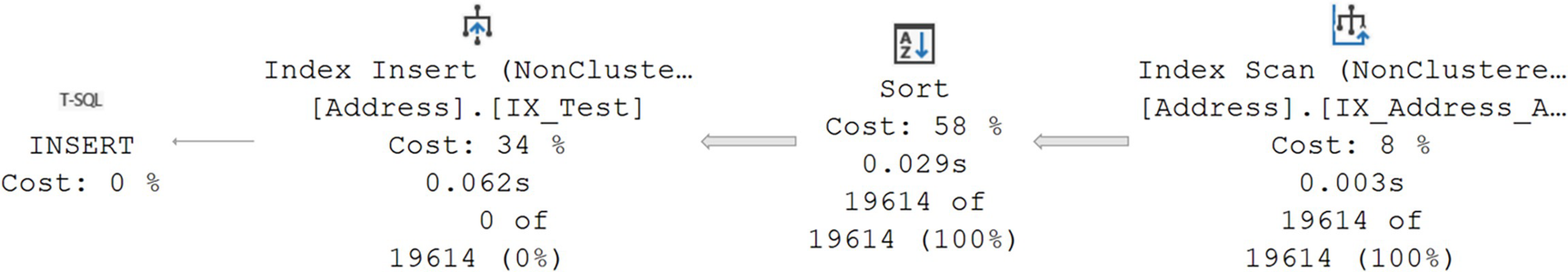
A diagram begins on the right with a non clustered index scan with values of, 8% cost, 0.003 seconds, and 19614 of 19614, given. From there it goes to sort on the left with values of 58%, 0.029 seconds, and 19614 of 19614.
The execution plan for a CREATE INDEX statement
Instead of scanning the clustered index to arrive at the data set, the optimizer chose in this case to scan the nonclustered index, IX_Address_AddressLine1_AddressLine2_City_StateProvinceID_PostalCode. Both the clustered index and the nonclustered index used contain all the City values, but the nonclustered index is smaller, so fewer pages need to be read while creating the index.
Parallel Index Creation
Just as queries can run in parallel, SQL Server can create indexes using parallel execution, but only on the Enterprise edition. If you have a multiprocessor machine supporting your SQL Server instance, you can put those processors to work when creating an index. You control the number of processors used at the server level by setting the “Max Degree of Parallelism”. You can also control it at the query level by using the MAXDOP query hint on your CREATE INDEX statement.
Online Index Creation
The default creation of an index is done as an offline operation. This means exclusive locks are placed on the table, restricting user access while the index is created. It is possible to create the indexes as an online operation. This allows users to continue to access the data while the index is being created. This comes at the cost of increasing the amount of time and resources it takes to create the index. Introduced in SQL Server 2012, indexes with varchar(MAX), nvarchar(MAX), and varbinary(MAX) can actually be rebuilt online. Online index operations are available only in SQL Server Enterprise editions.
Considering the Database Engine Tuning Advisor
SQL Server has a tool called the Database Engine Tuning Advisor. In previous editions of the book, I dedicated a chapter to this. However, over the years I’ve lost more and more faith in the tool. Now, I never use it and won’t advocate for its use. However, in some cases, people have found it to be helpful in deciding which indexes to apply to their systems. I will add that some of its suggestions are not helpful. Some of its suggestions may even be harmful. If you do choose to use the Tuning Advisor, please do extensive testing to validate its results.
OPTIMIZE_FOR_SEQUENTIAL_KEY
When you have an index on a value that is sequential, it’s very common to see contention in the last page of the index, as multiple processes all attempt to insert values to the same page. Common values would be an IDENTITY column, a date or time column, or an ordered GUID. Starting with SQL Server 2019, and available in Azure SQL Database, you can enable OPTIMIZE_FOR_SEQUENTIAL_KEY. It will change the way the inserts occur in order to reduce the last page contention. You may also see this help other indexes that are experiencing similar contention.
Resumable Indexes and Constraints
Creating an index that can be paused
The RESUMABLE option is part of the ONLINE index functionality, so you’ll need to include both. Not only does this make it possible to pause the rebuild of an index while leaving the index in place, but you can restart failed index rebuilds. It’s a handy function. You can also add MAX_DURATION to the command in order to have it pause automatically after a number of minutes.
Getting information on paused index rebuilds
Pausing an index rebuild
Code to restart or abort an index rebuild
This does incur some disk storage overhead since the partially built index needs to be kept somewhere. Plan for at least as much storage as the index currently takes up. Using RESUMABLE means that you can’t use SORT_IN_TEMPDB. Finally, you can’t run a RESUMABLE index operation within an explicit transaction.
Special Index Types
As special data types and storage mechanisms are introduced to SQL Server by Microsoft, methods for indexing these special storage types are also developed. Explaining all the details possible for each of these special index types is outside the scope of the book. In the following sections, I introduce the basic concepts of each index type in order to facilitate the possibility of their use in tuning your queries.
Full-Text
You can store large amounts of text in SQL Server by using the MAX value in the VARCHAR, NVARCHAR, CHAR, and NCHAR fields. A normal clustered or nonclustered index against these large fields would be unsupportable because a single value can far exceed the page size within an index. So a different mechanism of indexing text is to use the full-text engine, which must be running to work with full-text indexes. You can also build a full-text index on VARBINARY data.
You need to have one column on the table that is unique. The best candidates for performance are integers: INT or BIGINT. This column is then used along with the word to identify which row within the table it belongs to, as well as its location within the field. SQL Server allows for incremental changes, either change tracking or time based, to the full-text indexes as well as complete rebuilds.
SQL Server 2012 introduced another method for working with text called Semantic Search. It uses phrases from documents to identify relationships between different sets of text stored within the database.
Spatial
Introduced in SQL Server 2008 is the ability to store spatial data. This data can be either a geometry type or the very complex geographical type, literally identifying a point on the earth. To say the least, indexing this type of data is complicated. SQL Server stores these indexes in a flat B-Tree, similar to regular indexes, except that it is also a hierarchy of four grids linked together. Each of the grids can be given a density of low, medium, or high, outlining how big each grid is. There are mechanisms to support indexing of the spatial data types so that different types of queries, such as finding when one object is within the boundaries or near another object, can benefit from performance increases inherent in indexing.
A spatial index can be created only against a column of type geometry or geography. It has to be on a base table, it must have no indexed views, and the table must have a primary key. You can create up to 249 spatial indexes on any given column on a table. Different indexes are used to define different types of index behavior.
XML
Introduced as a data type in SQL Server 2005, XML can be stored not as text but as well-formed XML data within SQL Server. This data can be queried using the XQuery language as supported by SQL Server. To enhance the performance capabilities, a special set of indexes has been defined. An XML column can have one primary and several secondary indexes. The primary XML shreds the properties, attributes, and elements of the XML data and stores it as an internal table. There must be a primary key on the table, and that primary key must be clustered in order to create an XML index. After the XML index is created, the secondary indexes can be created. These indexes have types Path, Value, and Property, depending on how you query the XML.
Summary
This chapter expanded on the capabilities, functions, and behaviors of the indexes that we introduced in the preceding chapter. Any, or all, of these can help improve performance on your systems, but be sure that you do test them, because they all come with some additional overhead.
In the next chapter, we’ll explore lookups in detail and talk about possible ways to improve performance around them.