Chapter 7

Analytics Using Complex Data Types

Learning Objectives

By the end of this chapter, you will be able to:

• Perform descriptive analytics on time series data using DATETIME
• Use geospatial data to identify relationships
• Use complex data types (arrays, JSON, and JSONB)
• Perform text analytics

This chapter covers how to make the most of your data by analyzing complex and alternative data types.

Introduction

In the previous chapter, we looked at how we can import and export data into other analytical tools in order to leverage analytical tools outside of our database. It is often easiest to analyze numbers, but in the real world, data is frequently found in other formats: words, locations, dates, and sometimes complex data structures. In this chapter, we will look at these other formats, and see how we can use this data in our analysis.

First, we will look at two commonly found column types: datetime columns and latitude and longitude columns. These data types will give us a foundational understanding of how to understand our data from both a temporal and a geospatial perspective. Next, we will look at complex data types, such as arrays and JSON, and learn how to extract data points from these complex data types. These data structures are often used for alternative data, or log-level data, such as website logs. Finally, we will look at how we can extract meaning out of text in our database and use text data to extract insights.

By the end of the chapter, you will have broadened your analysis capabilities so that you can leverage just about any type of data available to you.

Date and Time Data Types for Analysis

We are all familiar with dates and times, but we don't often think about how these quantitative measures are represented. Yes, they are represented using numbers, but not with a single number. Instead, they are measured with a set of numbers, one for the year, one for the month, one for the day of the month, one for the hour, one for the minute, and so on.

What we might not realize, though, is that this is a complex representation, comprising several different components. For example, knowing the current minute without knowing the current hour is useless. Additionally, there are complex ways of interacting with dates and times, for example, different points in time can be subtracted from one another. Additionally, the current time can be represented differently depending on where you are in the world.

As a result of these intricacies, we need to take special care when working with this type of data. In fact, Postgres, like most databases, offers special data types that can represent these types of values. We'll start by examining the date type.

Starting with the Date Type

Dates can be easily represented using strings, for example, "January 1, 2000," which clearly represents a specific date, but dates are a special form of text in that they represent a quantitative and sequential value. You can add a week to the current date, for example. A given date has many different properties that you might want to use in your analysis, for instance, the year or the day of the week that the date represents. Working with dates is also necessary for time series analysis, which is one of the most common types of analysis that come up.

The SQL standard includes a DATE data type, and PostgreSQL offers great functionality for interacting with this data type. First, we can set our database to display dates in the format that we are most familiar with. PostgreSQL uses the DateStyle parameter to configure these settings. To see your current settings, you can use the following command:

SHOW DateStyle;

The following is the output of the preceding query:

Figure 7.1: Displaying the current DateStyle configuration

The first parameter specifies the International Organization Standardization (ISO) output format, which displays the date as Year, Month, Day and the second parameter specifies the ordering (for example, Month, Day, Year versus Day, Month, Year) for input or output. You can configure the output for your database using the following command:

SET DateStyle='ISO, MDY';

For example, if you wanted to set it to the European format of Day, Month, Year, you would set DateStyle to 'GERMAN, DMY'. For this chapter, we will use the ISO display format (Year, Month, Day) and the Month, Day, Year input format. You can configure this format by using the preceding command.

Let's start by testing out the date format:

# SELECT '1/8/1999'::DATE;

    date    

------------

1999-01-08

(1 row)

As we can see, when we input a string, '1/8/1999', using the Month, Day, Year format, Postgres understands that this is January 8, 1999 (and not August 1, 1999). It displays the date using the ISO format specified previously, in the form YYYY-MM-DD.

Similarly, we could use the following formats with dashes and periods to separate the date components:

# SELECT '1-8-1999'::DATE;

    date    

------------

1999-01-08

(1 row)

# SELECT '1.8.1999'::DATE;

    date    

------------

1999-01-08

(1 row)

In addition to displaying dates that are input as strings, we can display the current date very simply using the current_date keywords in Postgres:

# SELECT current_date;

current_date

--------------

2019-04-28

(1 row)

In addition to the DATE data type, the SQL standard offers a TIMESTAMP data type. A timestamp represents a date and a time, down to a microsecond.

We can see the current timestamp using the now() function, and we can specify our time zone using AT TIME ZONE 'UTC'. Here's an example of the now() function with the Eastern Standard time zone specified:

# SELECT now() AT TIME ZONE 'EST';

          timezone          

----------------------------

2019-04-28 13:47:44.472096

(1 row)

We can also use the timestamp data type without time zone specified. You can grab the current time zone with the now() function:

# SELECT now();

              now              

-------------------------------

2019-04-28 19:16:31.670096+00

(1 row)

Note

In general, it is recommended that you use a timestamp with the time zone specified. If you do not specify the time zone, the value of the timestamp could be questionable (for example, the time could be represented in the time zone where the company is located, in Universal Time Coordinated (UTC) time, or the customer's time zone).

The date and timestamp data types are helpful not only because they display dates in a readable format, but also because they store these values using fewer bytes than the equivalent string representation (a date type value requires only 4 bytes, while the equivalent text representation might be 8 bytes for an 8-character representation such as '20160101'). Additionally, Postgres provides special functionality to manipulate and transform dates, and this is particularly useful for data analytics.

Transforming Date Types

Often, we will want to decompose our dates into their component parts. For example, we may be interested in only the year and month, but not the day, for the monthly analysis of our data. To do this, we can use EXTRACT(component FROM date). Here's an example:

# SELECT current_date,

    EXTRACT(year FROM current_date) AS year,

    EXTRACT(month FROM current_date) AS month,

    EXTRACT(day FROM current_date) AS day;

current_date | year | month | day

--------------+------+-------+-----

2019-04-28   | 2019 |     4 |  28

(1 row)

Similarly, we can abbreviate these components as y, mon, and d, and Postgres will understand what we want:

# SELECT current_date,

    EXTRACT(y FROM current_date) AS year,

    EXTRACT(mon FROM current_date) AS month,

    EXTRACT(d FROM current_date) AS day;

current_date | year | month | day

--------------+------+-------+-----

2019-04-28   | 2019 |     4 |  28

(1 row)

In addition to the year, month, and day, we will sometimes want additional components, such as day of the week, week of the year, or quarter. You can also extract these date parts as follows:

# SELECT current_date,

    EXTRACT(dow FROM current_date) AS day_of_week,

    EXTRACT(week FROM current_date) AS week_of_year,

    EXTRACT(quarter FROM current_date) AS quarter;

current_date | day_of_week | week | quarter

--------------+-------------+------+---------

2019-04-28   |           0 |   17 |       2

(1 row)

Note that EXTRACT always outputs a number, so in this case, day_of_week starts at 0 (Sunday) and goes up to 6 (Saturday). Instead of dow, you can use isodow, which starts at 1 (Monday) and goes up to 7 (Sunday).

In addition to extracting date parts from a date, we may want to simply truncate our date or timestamp. For example, we may want to simply truncate our date to the year and month. We can do this using the DATE_TRUNC() function:

[datalake] # SELECT NOW(), DATE_TRUNC('month', NOW());

              now              |       date_trunc      

-------------------------------+------------------------

2019-04-28 19:40:08.691618+00 | 2019-04-01 00:00:00+00

(1 row)

Notice that the DATE_TRUNC (...) function does not round off the value. Instead, it outputs the greatest rounded value less than or equal to the date value that you input.

Note

The DATE_TRUNC(…) function is similar to the flooring function in mathematics, which outputs the greatest integer less than or equal to the input (for example, 5.7 would be floored to 5).

The DATE_TRUNC (...) function is particularly useful for GROUP BY statements. For example, you can use it to group sales by quarter, and get the total quarterly sales:

SELECT DATE_TRUNC('quarter', NOW()) AS quarter,

    SUM(sales_amount) AS total_quarterly_sales

FROM sales

GROUP BY 1

ORDER BY 1 DESC;

Note

DATE_TRUNC(…) requires a string representing the field you want to truncate to, while EXTRACT(…) accepts either the string representation (with quotes) or the field name (without quotes).

Intervals

In addition to representing dates, we can also represent fixed time intervals using the interval data type. This is useful if we want to analyze how long something takes, for example, if we want to know how long it takes a customer to make a purchase.

Here's an example:

# SELECT INTERVAL '5 days';

interval

----------

5 days

(1 row)

Intervals are useful for subtracting timestamps, for example:

# SELECT TIMESTAMP '2016-03-01 00:00:00' - TIMESTAMP '2016-02-01 00:00:00' AS days_in_feb;

days_in_feb

-------------

29 days

(1 row)

Or, alternatively, intervals can be used to add the number of days to a timestamp:

# SELECT TIMESTAMP '2016-03-01 00:00:00' + INTERVAL '7 days' AS new_date;

      new_date      

---------------------

2016-03-08 00:00:00

(1 row)

While intervals offer a precise method for doing timestamp arithmetic, the DATE format can be used with integers to accomplish a similar result. In the following example, we simply add 7 (an integer) to the date to calculate the new date:

# SELECT DATE '2016-03-01' + 7 AS new_date;

  new_date  

------------

2016-03-08

(1 row)

Similarly, we can subtract two dates and get an integer result:

# SELECT DATE '2016-03-01' - DATE '2016-02-01' AS days_in_feb;

days_in_feb

-------------

          29

(1 row)

While the date data type offers ease of use, the timestamp with the time zone data type offers precision. If you need your date/time field to be precisely the same as the time at which the action occurred, you should use the timestamp with the time zone. If not, you can use the date field.

Exercise 22: Analytics with Time Series Data

In this exercise, we will perform basic analysis using time series data to derive insights into how ZoomZoom has ramped up its efforts to sell more vehicles during the year 2018 by using the ZoomZoom database.

Note

All the exercises and activity codes of this chapter can also be found on GitHub: https://github.com/TrainingByPackt/SQL-for-Data-Analytics/tree/master/Lesson07.

Perform the following steps to complete the exercise:

1. First, let's look at the number of monthly sales. We can use the following aggregate query using the DATE_TRUNC method:

   SELECT

       DATE_TRUNC('month', sales_transaction_date)

           AS month_date,

       COUNT(1) AS number_of_sales

   FROM sales

   WHERE EXTRACT(year FROM sales_transaction_date) = 2018

   GROUP BY 1

   ORDER BY 1;

   After running this SQL, we get the following result:

   

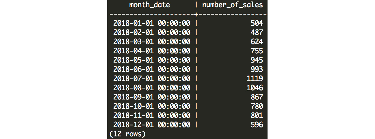
   Figure 7.2: Monthly number of sales

2. Next, we can look at how this compares with the number of new customers joining each month:

   SELECT

       DATE_TRUNC('month', date_added)

           AS month_date,

       COUNT(1) AS number_of_new_customers

   FROM customers

   WHERE EXTRACT(year FROM date_added) = 2018

   GROUP BY 1

   ORDER BY 1;

   The following is the output of the preceding query:

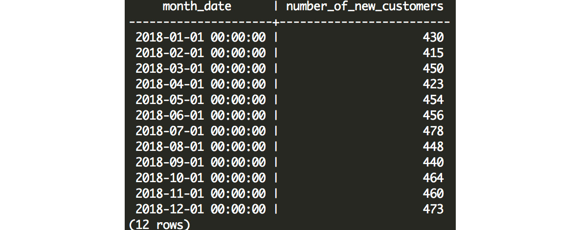
Figure 7.3: Number of new customer sign-ups every month

We can probably deduce that customers are not being entered into our database during their purchase, but instead, they are signing up with us before they make a purchase. The flow of new potential customers is fairly steady, and hovers around 400-500 new customer sign-ups every month, while the number of sales (as queried in step 1) varies considerably – in July, we have 2.3 times as many sales (1,119) as we have new customers (478).

From this exercise, we can see that we get a steady number of customers entering our database, but sales transactions vary considerably from month to month.

Performing Geospatial Analysis in Postgres

In addition to looking at time series data to better understand trends, we can also use geospatial information – such as city, country, or latitude and longitude – to better understand our customers. For example, governments use geospatial analysis to better understand regional economic differences, while a ride-sharing platform might use geospatial data to find the closest driver for a given customer.

We can represent a geospatial location using latitude and longitude coordinates, and this will be the fundamental building block for us to begin geospatial analysis.

Latitude and Longitude

When we think about locations, we often think about it in terms of the address – the city, state, country, or postal code that is assigned to the location that we are interested in. From an analytics perspective, this is sometimes OK – for example, you can look at the sales volume by city and come up with meaningful results about which cities are performing well.

Often, however, we need to understand geospatial relationships numerically, to understand the distances between two points, or to understand relationships that vary based on where you are on a map. After all, if you live on the border between two cities, it's rare that your behavior would suddenly change if you move to the other city.

Latitude and longitude allow us to look at the location in a continuous context. This allows us to analyze the numeric relationships between location and other factors (for example, sales). latitude and longitude also enable us to look at the distances between two locations.

Latitude tells us how far north or south a point is. A point at +90° latitude is at the North Pole, while a point at 0° latitude is at the equator, and a point at -90° is at the South Pole. On a map, lines of constant latitude run east and west.

Longitude tells us how far east, or west, a point is. On a map, lines of constant latitude run east and west. Greenwich, England, is the point of 0° longitude. Points can be defined using longitude as west (-) or east (+) of this point, and values range from -180° west to +180° east. These values are actually equivalent because they both point to the vertical line that runs through the Pacific Ocean, which is halfway around the world from Greenwich, England.

Representing Latitude and Longitude in Postgres

In Postgres, we can represent latitude and longitude using two floating-point numbers. In fact, this is how latitude and longitude are represented in the ZoomZoom customers table:

SELECT

    latitude,

    longitude

FROM customers

LIMIT 10;

Here is the output of the preceding query:

Figure 7.4: Latitudes and longitudes of ZoomZoom customers

Here, we can see that all of the latitudes are positive because the United States is north of the equator. All of the longitudes are negative because the United States is west of Greenwich, England. We can also see that some customers do not have latitude and longitude values filled in, because their location is unknown.

While these values can give us the exact location of a customer, we cannot do much with that information, because distance calculations require trigonometry, and make simplifying assumptions about the shape of the Earth.

Thankfully, Postgres has tools to solve this problem. We can calculate distances in Postgres by installing these packages:

CREATE EXTENSION cube;

CREATE EXTENSION earthdistance;

These two extensions only need to be installed once, by running the two preceding commands. The earthdistance module depends on the cube module. Once we install the earthdistance module, we can define a point:

SELECT

    point(longitude, latitude)

FROM customers

LIMIT 10;

Here is the output of the preceding query:

Figure 7.5: Customer latitude and longitude represented as points in Postgres

Note

A point is defined with longitude first and then latitude. This is contrary to the convention of latitude first and then longitude. The rationale behind this is that longitude more closely represents points along an x-axis, and latitude more closely represents points on the y-axis, and in mathematics, graphed points are usually noted by their x coordinate followed by their y coordinate.

The earthdistance module also allows us to calculate the distance between points in miles:

SELECT

    point(-90, 38) <@> point(-91, 37) AS distance_in_miles;

Here is the output of the preceding query:

Figure 7.6: The distance (in miles) between two points separated by 1° longitude and 1° latitude

In this example, we defined two points, (38° N, 90° W) and (37° N, 91° W), and we were able to calculate the distance between these points using the <@> operator, which calculates the distance in miles (in this case, these two points are 88.2 miles apart).

In the following exercise, we will see how we can use these distance calculations in a practical business context.

Exercise 23: Geospatial Analysis

In this exercise, we will identify the closest dealership for each customer. ZoomZoom marketers are trying to increase customer engagement by helping customers find their nearest dealership. The product team is also interested to know what the average distance is between each customer and their closest dealership.

Follow these steps to implement the exercise:

1. First, we will create a table with the longitude and latitude points for every customer:

   CREATE TEMP TABLE customer_points AS (

       SELECT

           customer_id,

           point(longitude, latitude) AS lng_lat_point

       FROM customers

       WHERE longitude IS NOT NULL

       AND latitude IS NOT NULL

   );

2. Next, we can create a similar table for every dealership:

   CREATE TEMP TABLE dealership_points AS (

       SELECT

           dealership_id,

           point(longitude, latitude) AS lng_lat_point

       FROM dealerships

   );

3. Now we can cross join these tables to calculate the distance from each customer to each dealership (in miles):

   CREATE TEMP TABLE customer_dealership_distance AS (

       SELECT

          customer_id,

          dealership_id,

          c.lng_lat_point <@> d.lng_lat_point AS distance

       FROM customer_points c

       CROSS JOIN dealership_points d

   );

4. Finally, we can take the closest dealership for each customer using the following query:

   CREATE TEMP TABLE closest_dealerships AS (

       SELECT DISTINCT ON (customer_id)

           customer_id,

           dealership_id,

           distance

       FROM customer_dealership_distance

       ORDER BY customer_id, distance

   );

   Remember that the DISTINCT ON clause guarantees only one record for each unique value of the column in parentheses. In this case, we will get one record for every customer_id, and because we sort by distance, we will get the record with the shortest distance.

5. Now that we have the data to fulfill the marketing team's request, we can now calculate the average distance from each customer to their closest dealership:

   SELECT

       AVG(distance) AS avg_dist,

       PERCENTILE_DISC(0.5) WITHIN GROUP (ORDER BY distance) AS median_dist

   FROM closest_dealerships;

   Here is the output of the preceding query:

Figure 7.7: Average and median distances between customers and their closest dealership

The result is that the average distance is about 147 miles away, but the median distance is about 91 miles.

In this exercise, we represented the geographic points for every customer, then calculated the distance for each customer and every possible dealership, identified the closest dealership for each customer, and found the average and median distances to a dealership for our customers.

Using Array Data Types in Postgres

While the Postgres data types that we have explored so far allow us to store many different types of data, occasionally we will want to store a series of values in a table. For example, we might want to store a list of the products that a customer has purchased, or we might want to store a list of the employee ID numbers associated with a specific dealership. For this scenario, Postgres offers the ARRAY data type, which allows us to store just that – a list of values.

Starting with Arrays

Postgres arrays allow us to store multiple values in a field in a table. For example, consider the following first record in the customers table:

customer_id        | 1

title              | NULL

first_name          | Arlena

last_name          | Riveles

suffix              | NULL

email              | [email protected]

gender             | F

ip_address         | 98.36.172.246

phone              | NULL

street_address     | NULL

city               | NULL

state              | NULL

postal_code        | NULL

latitude           | NULL

longitude          | NULL

date_added         | 2017-04-23 00:00:00

Each field contains exactly one value (the NULL value is still a value); however, there are some attributes that might contain multiple values with an unspecified length. For example, imagine that we wanted to have a purchased_products field. This could contain zero or more values within the field. For example, imagine the customer purchased the Lemon and Bat Limited Edition scooters; we can represent that as follows:

purchased_products | {Lemon,"Bat Limited Edition"}

We can define an array in a variety of ways. To get started, we can simply create an array using the following command:

SELECT ARRAY['Lemon', 'Bat Limited Edition'] AS example_purchased_products;

  example_purchased_products  

-------------------------------

{Lemon,"Bat Limited Edition"}

Postgres knows that the 'Lemon' and 'Bat Limited Edition' values are of the text data type, so it creates a text array to store these values.

While you can create an array for any data type, the array is limited to values for that data type only. So, you could not have an integer value followed by a text value (this would likely produce an error).

We can also create arrays using the ARRAY_AGG aggregate function. For example, the following query aggregates all of the vehicles for each product type:

SELECT product_type, ARRAY_AGG(DISTINCT model) AS models FROM products GROUP BY 1;

The following is the output of the preceding query:

Figure 7.8: Output of the ARRAY_AGG function

You can also reverse this operation using the UNNEST function, which creates one row for every value in the array:

SELECT UNNEST(ARRAY[123, 456, 789]) AS example_ids;

Here is the output of the preceding query:

Figure 7.9: Output of the UNNEST command

You can also create an array by splitting a string value using the STRING_TO_ARRAY function. Here's an example:

SELECT STRING_TO_ARRAY('hello there how are you?', ' ');

In this example, the sentence is split using the second string (' '), and we end up with the result:

Figure 7.10: A string value is split into an array of strings

Similarly, we can run the reverse operation, and concatenate an array of strings into a single string:

SELECT ARRAY_TO_STRING(ARRAY['Lemon', 'Bat Limited Edition'], ', ')  AS example_purchased_products;

In this example, we can join the individual string with the second string using ', ':

Figure 7.11: A new string is formed from an array of strings

There are other functions that allow you to interact with arrays. Here are a few examples of the additional array functionality that Postgres provides:

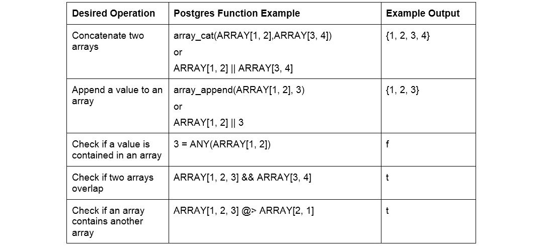
Figure 7.12: Examples of additional array functionality

Using JSON Data Types in Postgres

While arrays can be useful for storing a list of values in a single field, sometimes our data structures can be complex. For example, we might want to store multiple values of different types in a single field, and we might want data to be keyed with labels rather than stored sequentially. These are common issues with log-level data, as well as alternative data.

JavaScript Object Notation (JSON) is an open standard text format for storing data of varying complexity. It can be used to represent just about anything. Similar to how a database table has column names, JSON data has keys. We can represent a record from our customers database easily using JSON, by storing column names as keys, and row values as values. The row_to_json function transforms rows to JSON:

SELECT row_to_json(c) FROM customers c limit 1;

Here is the output of the preceding query:

{"customer_id":1,"title":null,"first_name":"Arlena","last_name":"Riveles","suffix":null,"email":"[email protected]","gender":"F","ip_address":"98.36.172.246","phone":null,"street_address":null,"city":null,"state":null,"postal_code":null,"latitude":null,"longitude":null,"date_added":"2017-04-23T00:00:00"}

This is a little hard to read, but we can add the pretty_bool flag to the row_to_json function to generate a readable version:

SELECT row_to_json(c, TRUE) FROM customers c limit 1;

Here is the output of the preceding query:

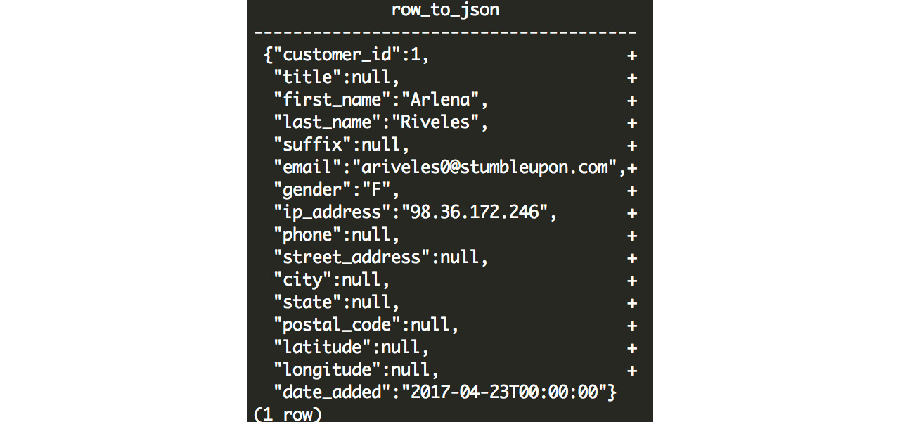
Figure 7.13: JSON output from row_to_json

As you can see, once we reformat the JSON, it presents a simple, readable, text representation of our row. The JSON structure contains keys and values. In this example, the keys are simply the column names, and the values come from the row values. JSON values can either be numeric values (either integers or floats), Boolean values (true or false), text values (wrapped with double quotation marks), or null.

JSON can also include nested data structures. For example, we can take a hypothetical scenario where we want to include purchased products in the table as well:

{

"customer_id":1,

"example_purchased_products":["Lemon", "Bat Limited Edition"]

}

Or, we can take this example one step further:

{                                                          

     "customer_id": 7,                                      

     "sales": [                                            

         {                                                  

             "product_id": 7,                              

             "sales_amount": 599.99,                        

             "sales_transaction_date": "2019-04-25T04:00:30"

         },                                                

         {                                                  

             "product_id": 1,                              

             "sales_amount": 399.99,                        

             "sales_transaction_date": "2011-08-08T08:55:56"

         },                                                

         {                                                  

             "product_id": 6,                              

             "sales_amount": 65500,                        

             "sales_transaction_date": "2016-09-04T12:43:12"

         }                                                  

     ],                                                    

}

In this example, we have a JSON object with two keys: customer_id and sales. As you can see, the sales key points to a JSON array of values, but each value is another JSON object representing the sale. JSON objects that exist within a JSON object are referred to as nested JSON. In this case, we have represented all of the sales transactions for a customer using a nested array that contains nested JSON objects for each sale.

While JSON is a universal format for storing data, it is inefficient, because everything is stored as one large text string. In order to retrieve a value associated with a key, you would need to first parse the text, and this has a relatively high computational cost associated with it. If you just have a few JSON objects, this performance overhead might not be a big deal; however, it might become a burden if, for example, you are trying to select the JSON object with "customer_id": 7 from millions of other JSON objects in your database.

In the next section, we will introduce JSONB, a binary JSON format, which is optimized for Postgres and allows you to avoid a lot of the parsing overhead associated with a standard JSON text string.

JSONB: Pre-Parsed JSON

While a text JSON field needs to be parsed each time it is referenced, a JSONB value is pre-parsed, and data is stored in a decomposed binary format. This requires that the initial input be parsed up front, and the benefit is that there is a significant performance improvement when querying the keys or values in this field. This is because the keys and values do not need to be parsed – they have already been extracted and stored in an accessible binary format.

Note

JSONB differs from JSON in a few other ways as well. First, you cannot have more than one key with the same name. Second, the key order is not preserved. Third, semantically insignificant details, such as whitespace, are not preserved.

Accessing Data from a JSON or JSONB Field

JSON keys can be used to access the associated value using the -> operator. Here's an example:

SELECT

    '{

         "a": 1,

         "b": 2,

         "c": 3

     }'::JSON -> 'b' AS data;

In this example, we had a three-key JSON value, and we are trying to access the value for the b key. The output is a single output: 2. This is because the -> 'b' operation gets the value for the b key from the JSON, {"a": 1, "b": 2, "c": 3}.

Postgres also allows more complex operations to access nested JSON using the #> operator. Take the following example:

SELECT

    '{

         "a": 1,

         "b": [

             {"d": 4},

             {"d": 6},

             {"d": 4}

    ],

         "c": 3

     }'::JSON #> ARRAY['b', '1', 'd'] AS data;

On the right side of the #> operator, a text array defines the path to access the desired value. In this case, we select the 'b' value, which is a list of nested JSON objects. Then, we select the element in the list denoted by '1', which is the second element because array indexes start at 0. Finally, we select the value associated with the 'd' key – and the output is 6.

These functions work with JSON or JSONB fields (keep in mind it will run much faster on JSONB fields). JSONB, however, also enables additional functionality. For example, let's say you want to filter rows based on a key-value pair. You could use the @> operator, which checks whether the JSONB object on the left contains the key value on the right. Here's an example:

SELECT * FROM customer_sales WHERE customer_json @> '{"customer_id":20}'::JSONB;

The preceding query outputs the corresponding JSONB record:

{"email": "[email protected]", "phone": null, "sales": [], "last_name": "Hughill", "date_added": "2012-08-08T00:00:00", "first_name": "Itch", "customer_id": 20}

With JSONB, we can also make our output look pretty using the jsonb_pretty function:

SELECT JSONB_PRETTY(customer_json) FROM customer_sales WHERE customer_json @> '{"customer_id":20}'::JSONB;

Here is the output of the preceding query:

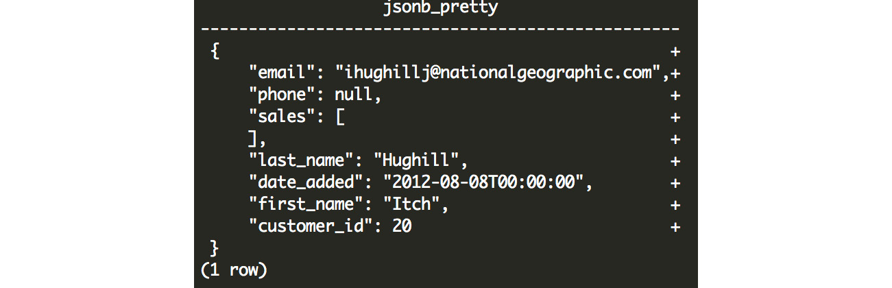
Figure 7.14: Output from the JSONB_PRETTY function

We can also select just the keys from the JSONB field, and unnest them into multiple rows using the JSONB_OBJECT_KEYS function. Using this function, we can also extract the value associated with each key from the original JSONB field using the -> operator. Here's an example:

SELECT

    JSONB_OBJECT_KEYS(customer_json) AS keys,

    customer_json -> JSONB_OBJECT_KEYS(customer_json) AS values

FROM customer_sales

WHERE customer_json @> '{"customer_id":20}'::JSONB

;

The following is the output of the preceding query:

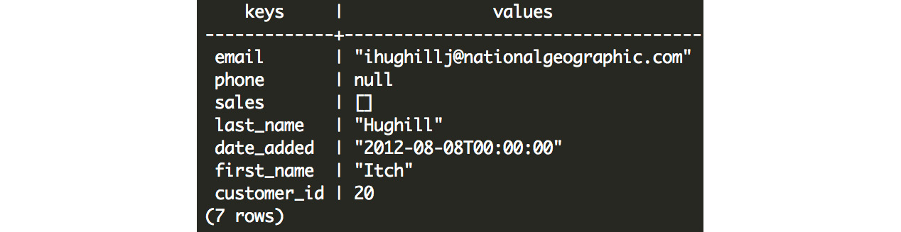
Figure 7.15: Keys and values pairs exploded into multiple rows using the JSONB_OBJECT_KEYS function

Creating and Modifying Data in a JSONB Field

You can also add and remove elements from JSONB. For example, to add a new key-value pair, "c": 2, you can do the following:

select jsonb_insert('{"a":1,"b":"foo"}', ARRAY['c'], '2');

Here is the output of the preceding query:

{"a": 1, "b": "foo", "c": 2}

If you wanted to insert values into a nested JSON object, you could do that too:

select jsonb_insert('{"a":1,"b":"foo", "c":[1, 2, 3, 4]}', ARRAY['c', '1'], '10');

This would return the following output:

{"a": 1, "b": "foo", "c": [1, 10, 2, 3, 4]}

In this example, ARRAY['c', '1'] represents the path where the new value should be inserted. In this case, it first grabs the 'c' key and corresponding array value, and then it inserts the value ('10') at position '1'.

To remove a key, you can simply subtract the key that you want to remove. Here's an example:

SELECT '{"a": 1, "b": 2}'::JSONB - 'b';

In this case, we have a JSON object with two keys: a and b. When we subtract b, we are left with just the a key and its associated value:

{"a": 1}

In addition to the methodologies described here, we might want to search through multiple layers of nested objects. We will learn this in the following exercise.

Exercise 24: Searching through JSONB

We will identify the values using data stored as JSNOB. Suppose we want to identify all customers who purchased a Blade scooter; we can do this using data stored as JSNOB.

Complete the exercise by implementing the following steps:

1. First, we need to explode out each sale into its own row. We can do this using the JSONB_ARRAY_ELEMENTS function, which does exactly that:

   CREATE TEMP TABLE customer_sales_single_sale_json AS (

       SELECT

           customer_json,

           JSONB_ARRAY_ELEMENTS(customer_json -> 'sales') AS sale_json

       FROM customer_sales LIMIT 10

   );

2. Next, we can simply filter this output, and grab the records where product_name is 'Blade':

   SELECT DISTINCT customer_json FROM customer_sales_single_sale_json WHERE sale_json ->> 'product_name' = 'Blade' ;

   The ->> operator is similar to the -> operator, except it returns text output rather than JSONB output. This outputs the following result:

   

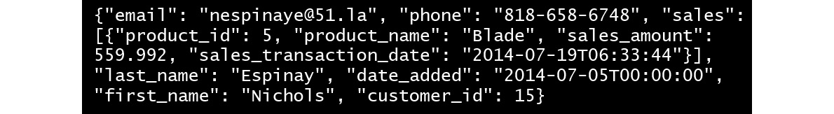
   Figure 7.16: Records where product_name is 'Blade'

3. We can make this result easier to read by using JSONB_PRETTY() to format the output:

   SELECT DISTINCT JSONB_PRETTY(customer_json) FROM customer_sales_single_sale_json WHERE sale_json ->> 'product_name' = 'Blade' ;

   Here is the output of the preceding query:

   

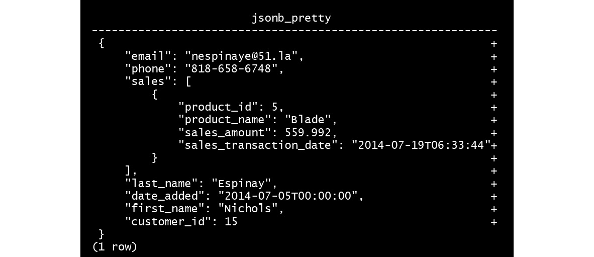
Figure 7.17: Format the output using JSNOB_PRETTY()

We can now easily read the formatted result after using the JSNOB_PRETTY() function.

In this exercise, we identified the values using data stored as JSNOB. We used JSNOB_PRETTY() and JSONB_ARRAY_ELEMENTS() to complete this exercise.

Text Analytics Using Postgres

In addition to performing analytics using complex data structures within Postgres, we can also make use of the non-numeric data available to us. Often, text contains valuable insights – you can imagine a salesperson keeping notes on prospective clients: "Very promising interaction, the customer is looking to make a purchase tomorrow" contains valuable data, as does this note: "The customer is uninterested. They no longer have a need for the product." While this text can be valuable for someone to manually read, it can also be valuable in the analysis. Keywords in these statements, such as "promising," "purchase," "tomorrow," "uninterested," and "no" can be extracted using the right techniques to try to identify top prospects in an automated fashion.

Any block of text can have keywords that can be extracted to uncover trends, for example, in customer reviews, email communications, or sales notes. In many circumstances, text data might be the most relevant data available, and we need to use it in order to create meaningful insights.

In this chapter, we will look at how we can use some Postgres functionality to extract keywords that will help us identify trends. We will also leverage text search capabilities in Postgres to enable rapid searching.

Tokenizing Text

While large blocks of text (sentences, paragraphs, and so on) can provide useful information to convey to a human reader, there are few analytical solutions that can draw insights from unprocessed text. In almost all cases, it is helpful to parse text into individual words. Often, the text is broken out into the component tokens, where each token is a sequence of characters that are grouped together to form a semantic unit. Usually, each token is simply a word in the sentence, although in certain cases (such as the word "can't"), your parsing engine might parse two tokens: "can" and "t".

Note

Even cutting-edge Natural Language Processing (NLP) techniques usually involve tokenization before the text can be processed. NLP can be useful to run analysis that requires a deeper understanding of the text.

Words and tokens are useful because they can be matched across documents in your data. This allows you to draw high-level conclusions at the aggregate level. For example, if we have a dataset containing sales notes, and we parse out the "interested" token, we can hypothesize that sales notes containing "interested" are associated with customers who are more likely to make a purchase.

Postgres has functionality that makes tokenization fairly easy. We can start by using the STRING_TO_ARRAY function, which splits a string into an array using a delimiter, for example, a space:

SELECT STRING_TO_ARRAY('Danny and Matt are friends.', ' ');

The following is the output of the preceding query:

{Danny,and,Matt,are,friends.}

In this example, the sentence Danny and Matt are friends. is split on the space character.

In this example, we have punctuation, which might be better off removed. We can do this easily using the REGEXP_REPLACE function. This function accepts four arguments: the text you want to modify, the text pattern that you want to replace, the text that should replace it, and any additional flags (most commonly, you will add the 'g' flag, specifying that the replacement should happen globally, or as many times as the pattern is encountered). We can remove the period using a pattern that matches the punctuation defined in the !@#$%^&*()-=_+,.<>/?|[] string and replaces it with space:

SELECT REGEXP_REPLACE('Danny and Matt are friends.', '[!,.?-]', ' ', 'g');

The following is the output of the preceding query:

Danny and Matt are friends

The punctuation has been removed.

Postgres also includes stemming functionality, which is useful for identifying the root stem of the token. For example, the tokens "quick" and "quickly" or "run" and "running" are not that different in terms of their meaning, and contain the same stem. The ts_lexize function can help us standardize our text by returning the stem of the word, for example:

SELECT TS_LEXIZE('english_stem', 'running');

The preceding code returns the following:

{run}

We can use these techniques to identify tokens in text, as we will see in the following exercise.

Exercise 25: Performing Text Analytics

In this exercise, we want to quantitatively identify keywords that correspond with higher-than-average ratings or lower-than-average ratings using text analytics. In our ZoomZoom database, we have access to some customer survey feedback, along with ratings for how likely the customer is to refer their friends to ZoomZoom. These keywords will allow us to identify key strengths and weaknesses for the executive team to consider in the future.

Follow these steps to complete the exercise:

1. Let's start by seeing what data we have:

   SELECT * FROM customer_survey limit 5;

   The following is the output of the preceding query:

   

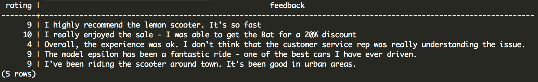
   Figure 7.18: Example customer survey responses in our database

   We can see that we have access to a numeric rating between 1 and 10, and feedback in text format.

2. In order to analyze the text, we need to parse it out into individual words and their associated ratings. We can do this using some array transformations:

   SELECT UNNEST(STRING_TO_ARRAY(feedback, ' ')) AS word, rating FROM customer_survey limit 10;

   The following is the output of the preceding query:

   

   Figure 7.19: Transformed text output

   As we can see from this output, the tokens are not standardized, and therefore this is problematic. In particular, punctuation (for example, It's), capitalization (for example, I and It's), word stems, and stop words (for example, I, the, and so) can be addressed to make the results more relevant.

3. Standardize the text using the ts_lexize function and using the English stemmer 'english_stem'. We will then remove characters that are not letters in our original text using REGEXP_REPLACE. Pairing these two functions together with our original query, we get the following:

   SELECT

       (TS_LEXIZE('english_stem',

                  UNNEST(STRING_TO_ARRAY(

                      REGEXP_REPLACE(feedback, '[^a-zA-Z]+', ' ', 'g'),

                      ' ')

                  )))[1] AS token,

       rating

   FROM customer_survey

   LIMIT 10;

   This returns the following:

   

   Figure 7.20: Output from TS_LEXIZE and REGEX_REPLACE

   Note

   When we apply these transformations, we call the outputs tokens rather than words. Tokens refer to each linguistic unit.

   Now we have the key tokens and their associated ratings available. Note that the output of this operation produces NULL values, so we will need to filter out those rating pairs.

4. In the next step, we will want to find the average rating associated with each token. We can actually do this quite simply using a GROUP BY clause:

   SELECT                                                                                      

       (TS_LEXIZE('english_stem',

                  UNNEST(STRING_TO_ARRAY(

                      REGEXP_REPLACE(feedback, '[^a-zA-Z]+', ' ', 'g'),

                      ' ')

                  )))[1] AS token,

       AVG(rating) AS avg_rating

   FROM customer_survey

   GROUP BY 1

   HAVING COUNT(1) >= 3

   ORDER BY 2

   ;

   In this query, we group by the first expression in the SELECT statement where we perform the tokenization. We can now take the average rating associated with each token. We want to make sure that we only take tokens with more than a couple of occurrences so that we can filter out the noise – in this case, due to the small sample size of feedback responses, we only require that the token occurs three or more times (HAVING COUNT(1) >= 3). Finally, we order the results by the second expression – the average score:

   

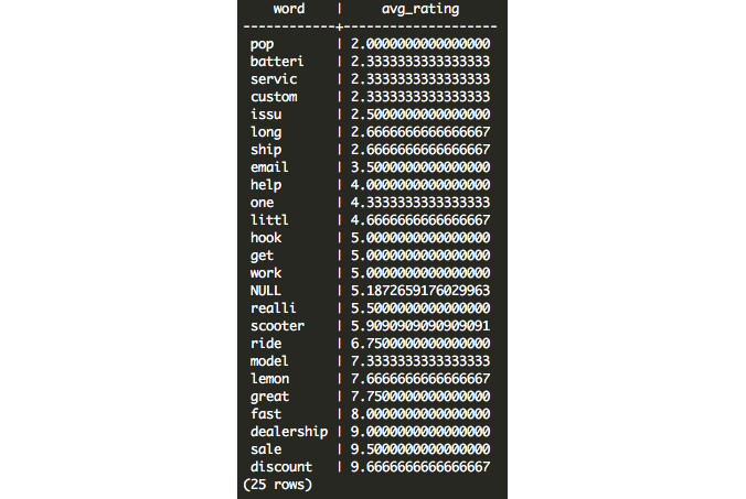
   Figure 7.21: Average ratings associated with text tokens

   On one end of the spectrum, we see that we have quite a few results that are negative: pop probably refers to popping tires, and batteri probably refers to issues with battery life. On the positive side, we see that customers respond favorably to discount, sale, and dealership.

5. Verify the assumptions by filtering survey responses that contain these tokens using an ILIKE expression, as follows:

   SELECT * FROM customer_survey WHERE feedback ILIKE '%pop%';

   This returns three relevant survey responses:

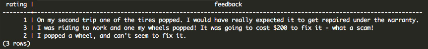
Figure 7.22: Filtering survey responses using ILIKE

The ILIKE expression allows us to match text that contains a pattern. In this example, we are trying to find text that contains the text pop, and the operation is case-insensitive. By wrapping this in % symbols, we are specifying that the text can contain any number of characters on the left or right.

Note

ILIKE is similar to another SQL expression: LIKE. The ILIKE expression is case-insensitive, and the LIKE expression is case-sensitive, so typically it will make sense to use ILIKE. In situations where performance is critical, LIKE might be slightly faster.

Upon receiving the results of our analysis, we can report the key issues to our product team to review. We can also report the high-level findings that customers like discounts and also feedback have been positive following the introduction of dealerships.

Performing Text Search

While performing text analytics using aggregations, as we did earlier, in some cases, it might be helpful instead to query our database for relevant posts, similar to how you might query a search engine.

While you can do this using an ILIKE expression in your WHERE clause, this is not terribly fast or extensible. For example, what if you wanted to search the text for multiple keywords, and what if you want to be robust to misspellings, or scenarios where one of the words might be missing altogether?

For these situations, we can use the text search functionality in Postgres. This functionality is pretty powerful and scales up to millions of documents when it is fully optimized.

Note

"Documents" represent the individual records in a search database. Each document represents the entity that we want to search for. For example, for a blogging website, this might be a blog article, which might include the title, the author, and the article for one blog entry. For a survey, it might include the survey responses, or perhaps the survey response combined with the survey question. A document can span multiple fields or even multiple tables.

We can start with the to_tsvector function, which will perform a similar function to the ts_lexize function. Rather than produce a token from a word, this will tokenize the entire document. Here's an example:

SELECT

    feedback,

    to_tsvector('english', feedback) AS tsvectorized_feedback

FROM customer_survey

LIMIT 1;

This produces the following result:

Figure 7.23: The tsvector tokenized representation of the original feedback

In this case, the feedback I highly recommend the lemon scooter. It's so fast was converted into a tokenized vector: 'fast':10 'high':2 'lemon':5 'recommend':3 'scooter':6. Similar to the ts_lexize function, less meaningful "stop words" were removed such as "I," "the," "It's," and "so." Other words, such as highly were stemmed to their root (high). Word order was not preserved.

The to_tsvector function can also take in JSON or JSONB syntax and tokenize the values (no keys) as a tsvector object.

The output data type from this operation is a tsvector data type. The tsvector data type is specialized and specifically designed for text search operations. In addition to tsvector, the tsquery data type is useful for transforming a search query into a useful data type that Postgres can use to search. For example, suppose we want to construct a search query with the lemon scooter keyword – we can write it as follows:

SELECT to_tsquery('english', 'lemon & scooter');

Or, if we don't want to specify the Boolean syntax, we can write it more simply as follows:

SELECT plainto_tsquery('english', 'lemon scooter');

Both of these produce the same result:

Figure 7.24: Transformed query with Boolean syntax

Note

to_tsquery accepts Boolean syntax, such as & for and and | for or. It also accepts ! for not.

You can also use Boolean operators to concatenate tsquery objects. For example, the && operator will produce a query that requires the left query and the right query, while the || operator will produce a query that matches either the left or the right tsquery object:

SELECT plainto_tsquery('english', 'lemon') && plainto_tsquery('english', 'bat') || plainto_tsquery('english', 'chi');

This produces the following result:

'lemon' & 'bat' | 'chi'

We can query a ts_vector object using a ts_query object using the @@ operator. For example, we can search all customer feedback for 'lemon scooter':

SELECT *

FROM customer_survey

WHERE to_tsvector('english', feedback) @@ plainto_tsquery('english', 'lemon scooter');

This returns the following three results:

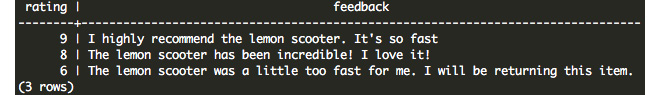
Figure 7.25: Search query output using the Postgres search functionality

Optimizing Text Search on Postgres

While the Postgres search syntax in the previous example is straightforward, it needs to convert all text documents into a tsvector object every time a new search is performed. Additionally, the search engine needs to check each and every document to see whether they match the query terms.

We can improve this in two ways:

• Store the tsvector objects so that they do not need to be recomputed.
• We can also store the tokens and their associated documents, similar to how an index in the back of a book has words or phrases and their associated page numbers so that we don't have to check each document to see whether it matches.

In order to do these two things, we will need to precompute and store the tsvector objects for each document and compute a Generalized Inverted Index (GIN).

In order to precompute the tsvector objects, we will use a materialized view. A materialized view is defined as a query, but unlike a regular view, where the results are queried every time, the results for a materialized view are persisted and stored as a table.

Because a materialized view stores results in a stored table, it can get out of sync with the underlying tables that it queries.

We can create a materialized view of our survey results using the following query:

CREATE MATERIALIZED VIEW customer_survey_search AS (

    SELECT

        rating,

        feedback,

        to_tsvector('english', feedback)

            || to_tsvector('english', rating::text) AS searchable

    FROM customer_survey

);

You can see that our searchable column is actually composed of two columns: the rating and feedback columns. There are many scenarios where you will want to search on multiple fields, and you can easily concatenate multiple tsvector objects together with the || operator.

We can test that the view worked by querying a row:

SELECT * FROM customer_survey_search LIMIT 1;

This produces the following output:

Figure 7.26: A record from our materialized view with tsvector

Whenever we need to refresh the view (for example, after an insert or update), we can use the following syntax:

REFRESH MATERIALIZED VIEW CONCURRENTLY customer_survey_search;

This will recompute the view concurrently while the old copy of the view remains available and unlocked.

Additionally, we can add the GIN index with the following syntax:

CREATE INDEX idx_customer_survey_search_searchable ON customer_survey_search USING GIN(searchable);

With these two operations (creating the materialized view and creating the GIN index), we can now easily query our feedback table using search terms:

SELECT rating, feedback FROM customer_survey_search WHERE searchable @@ plainto_tsquery('dealership');

The following is the output of the preceding query:

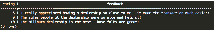
Figure 7.27: Output from the materialized view optimized for search

While the query time improvement might be small or non-existent for a small table of 32 rows, these operations greatly improve the speed for large tables (for example, with millions of rows), and enable users to quickly search their database in a matter of seconds.

Activity 9: Sales Search and Analysis

The head of sales at ZoomZoom has identified a problem: there is no easy way for the sales team to search for a customer. Thankfully, you volunteered to create a proof-of-concept internal search engine that will make all customers searchable by their contact information and the products that they have purchased in the past:

1. Using the customer_sales table, create a searchable materialized view with one record per customer. This view should be keyed off of the customer_id column and searchable on everything related to that customer: name, email, phone, and purchased products. It is OK to include other fields as well.
2. Create a searchable index on the materialized view that you created.
3. A salesperson asks you by the water cooler if you can use your new search prototype to find a customer by the name of Danny who purchased the Bat scooter. Query your new searchable view using the "Danny Bat" keywords. How many rows did you get?
4. The sales team wants to know how common it is for someone to buy a scooter and an automobile. Cross join the product table on itself to get all distinct pairs of products and remove pairs that are the same (for example, if the product name is the same). For each pair, search your view to see how many customers were found to match both products in the pair. You can assume that limited-edition releases can be grouped together with their standard model counterpart (for example, Bat and Bat Limited Edition can be considered the same scooter).

Expected Output:

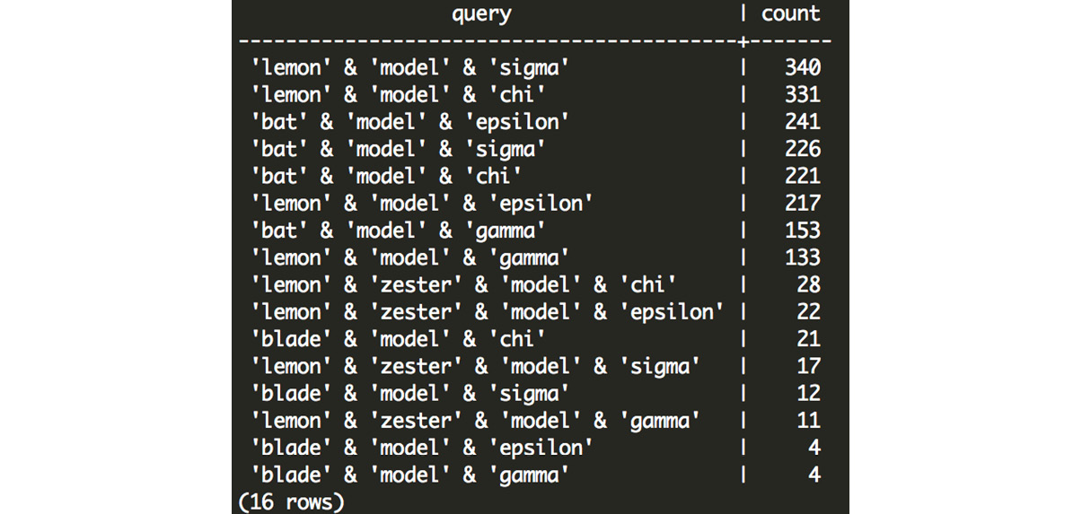
Figure 7.28: Customer counts for each scooter and automobile combination

Note

The solution for the activity can be found on page 336.

In this activity, we searched and analyzed the data using the materialized view. Then, we used DISTINCT and JOINS to transform the query. Lastly, we learned how to query our database using tsquery objects to get the final output.

Summary

In this chapter, we covered special data types including dates, timestamps, latitude and longitude, arrays, JSON and JSONB, and text data types. We learned how to transform these data types using specialized functionality for each data type, and we learned how we can perform advanced analysis using these data types and proved that this can be useful in a business context.

As our datasets grow larger and larger, these complex analyses become slower and slower. In the next chapter, we will take a deep look at how we can begin to optimize these queries using an explanation and analysis of the query plan, and using additional tools, such as indexes, that can speed up our queries.