Chapter 5

Window Functions for Data Analysis

Learning Objectives

By the end of this chapter, you will be able to:

• Explain what a window function is
• Write basic window functions
• Use common window functions to calculate statistics
• Analyze sales data using window functions and a window frame

In this chapter, we will cover window functions, functions similar to an aggregate function but that allow a new range of capabilities and insights.

Introduction

In the previous chapter, we discussed aggregate functions, functions that can take a large group of rows and output a single value for them. Often, being able to summarize a group of rows to a single value is important and useful. However, there are times when you want to keep the individual rows as well as gaining a summarizing value. To do this, in this chapter, we will introduce a new set of functions named window functions, which can calculate aggregate statistics while keeping individual rows. These functions are very useful for being able to calculate new types of statistics, such as ranks and rolling averages, with relative ease within SQL. In this chapter, we will learn about what window functions are, and how we can use them to calculate statistics.

Window Functions

Aggregate functions allow us to take many rows and convert those rows into one number. For example, the COUNT function takes in the rows of a table and returns the number of rows there are. However, we sometimes want to be able to calculate multiple rows but still keep all the rows following the calculation. For example, let's say you wanted to rank every user in order according to the time they became a customer, with the earliest customer being ranked 1, the second-earliest customer being ranked 2, and so on. You can get all the customers using the following query:

SELECT *

FROM customers

ORDER BY date_added;

You can order customers from the earliest to the most recent, but you can't assign them a number. You can use an aggregate function to get the dates and order them that way:

SELECT date_added, COUNT(*)

FROM customers

GROUP BY date_added

ORDER BY date_added

The following is the output of the preceding code:

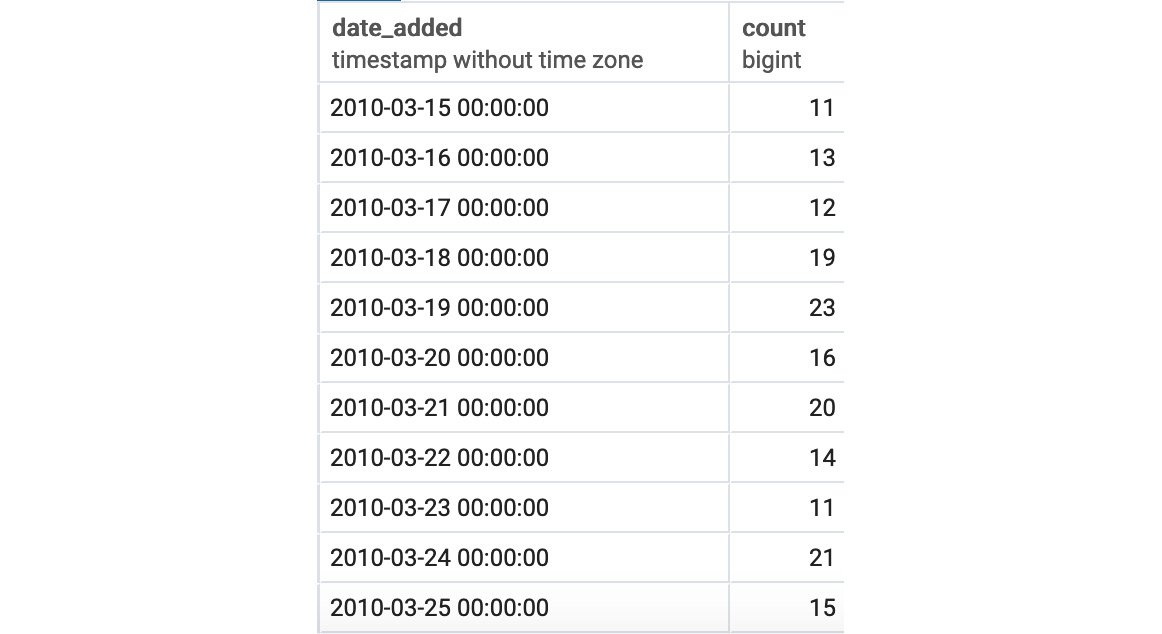
Figure 5.1: Aggregate date-time ordering

While this gives the dates, it gets rid of the remainder of the columns, and still provides no rank information. What can we do? This is where window functions come into play. Window functions can take multiple rows of data and process them, but still retain all the information in the rows. For things such as ranks, this is exactly what you need.

For better understanding though, let's see what a windows function query looks like in the next section.

The Basics of Window Functions

The following is the basic syntax of a window function:

SELECT {columns},

{window_func} OVER (PARTITION BY {partition_key} ORDER BY {order_key})

FROM table1;

Where {columns} are the columns to retrieve from tables for the query, {window_func} is the window function you want to use, {partition_key} is the column or columns you want to partition on (more on this later), {order_key} is the column or columns you want to order by, and table1 is the table or joined tables you want to pull data from. The OVER keyword indicates where the window definition starts.

To illustrate, let's use an example. You might be saying to yourself that you do not know any window functions, but the truth is, you do! All aggregate functions can be used as window functions. Let's use COUNT(*) in the following query:

SELECT customer_id, title, first_name, last_name, gender,

COUNT(*) OVER () as total_customers

FROM customers

ORDER BY customer_id;

This leads to the following results:

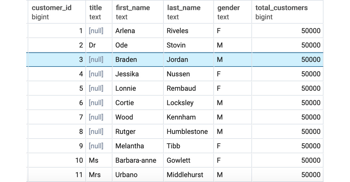
Figure 5.2: Customers listed using the COUNT(*) window query

As can be seen in Figure 5.2, the customers query returns title, first_name, and last_name, just like a typical SELECT query. However, there is now a new column called total_customers. This column contains the count of users that would be created by the following query:

SELECT COUNT(*)

FROM customers;

This returns 50,000. As discussed, the query returned both all of the rows and the COUNT(*) in the query, instead of just returning the count as a normal aggregate function would.

Now, let's examine the other parameters of the query. What happens if we use PARTITION BY, such as in the following query?

SELECT customer_id, title, first_name, last_name, gender,

COUNT(*) OVER (PARTITION BY gender) as total_customers

FROM customers

ORDER BY customer_id;

The following is the output of the preceding code:

Figure 5.3: Customers listed using COUNT(*) partitioned by the gender window query

Here, you will see that total_customers have now changed counts to one of two values, 24,956 or 25,044. These counts are the counts for each gender, which you can see with the following query:

SELECT gender, COUNT(*)

FROM customers

GROUP BY 1

For females, the count is equal to the female count, and for males, the count is equal to the male count. What happens now if we use ORDER BY in the partition, as follows?

SELECT customer_id, title, first_name, last_name, gender,

COUNT(*) OVER (ORDER BY customer_id) as total_customers

FROM customers

ORDER BY customer_id;

The following is the output of the preceding code:

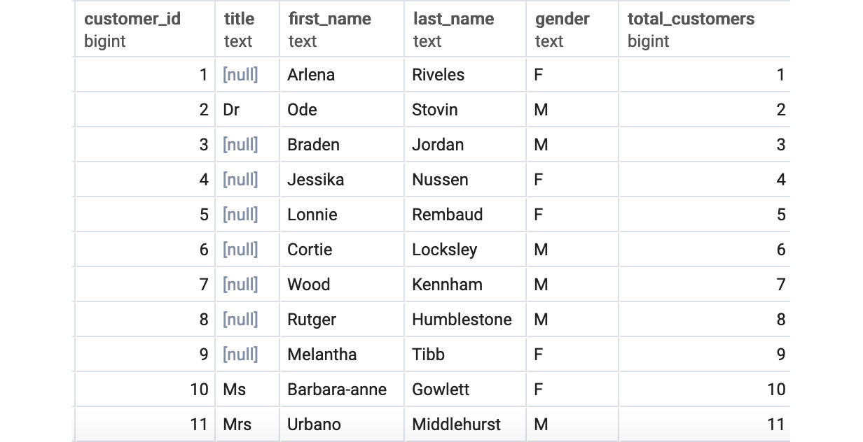
Figure 5.4: Customers listed using COUNT(*) ordered by the customer_id window query

You will notice something akin to a running count for total customers. What is going on? This is where the "window" in window function comes from. When you use a window function, the query creates a "window" over the table on which it bases the count. PARTITION BY works like GROUP BY, dividing the dataset into multiple groups. For each group, a window is created. When ORDER BY is not specified, the window is assumed to be the entire group. However, when ORDER BY is specified, the rows in the group are ordered according to it, and for every row, a window is created over which a function is applied. Without specifying a window, the default behavior is to create a window to encompass every row from the first row based on ORDER BY to the current row being evaluated by a function, as shown in Figure 5.5. It is over this window that the function is applied.

As shown in Figure 5.5, the window for the first row contains one row and returns a count of 1, the window for the second row contains two rows and returns a count of 2, whereas the window for the third row contains three rows and thus returns a count of 3 in the total_customers column:

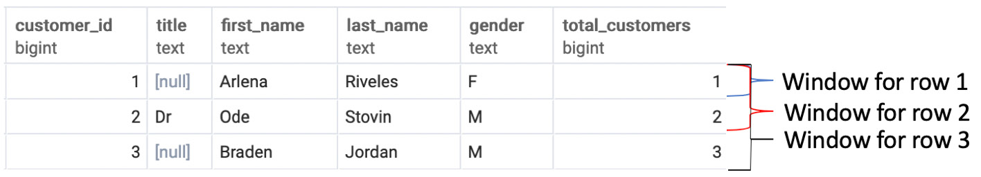
Figure 5.5: Windows for customers using COUNT(*) ordered by the customer_id window query

What happens when you combine PARTITION BY and ORDER BY? Let's look at the following query:

SELECT customer_id, title, first_name, last_name, gender,

COUNT(*) OVER (PARTITION BY gender ORDER BY customer_id) as total_customers

FROM customers

ORDER BY customer_id;

When you run the preceding query, you get the following result:

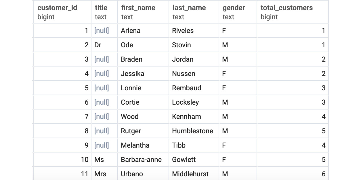
Figure 5.6: Customers listed using COUNT(*) partitioned by gender ordered by the customer_id window query

Like the previous query we ran, it appears to be some sort of rank. However, it seems to differ based on gender. What is this query doing? As discussed for the previous query, the query first divides the table into two subsets based on PARTITION BY. Each partition is then used as a basis for doing a count, with each partition having its own set of windows.

This process is illustrated in Figure 5.7. This process produces the count we see in Figure 5.7. The three keywords, OVER(), PARTITION BY, and ORDER BY, create the foundation to unlock the power of WINDOW functions.

Figure 5.7: Windows for customers listed using COUNT(*) partitioned by gender ordered by the customer_id window query

Exercise 16: Analyzing Customer Data Fill Rates over Time

For the last 6 months, ZoomZoom has been experimenting with various features in order to encourage people to fill out all fields on the customer form, especially their address. To analyze this data, the company would like a running total of how many users have filled in their street address over time. Write a query to produce these results.

Note

For all exercises in this chapter, we will be using pgAdmin 4. All the exercise and activities in this chapter are also available on GitHub: https://github.com/TrainingByPackt/SQL-for-Data-Analytics/tree/master/Lesson05.

1. Open your favorite SQL client and connect to the sqlda database.
2. Use window functions and write a query that will return customer information and how many people have filled out their street address. Also, order the list as per the date. The query would look like:

   SELECT customer_id, street_address, date_added::DATE,COUNT(CASE WHEN street_address IS NOT NULL THEN customer_id ELSE NULL END)

       OVER (ORDER BY date_added::DATE) as total_customers_filled_street

   FROM customers

   ORDER BY date_added;

   You should get the following result:

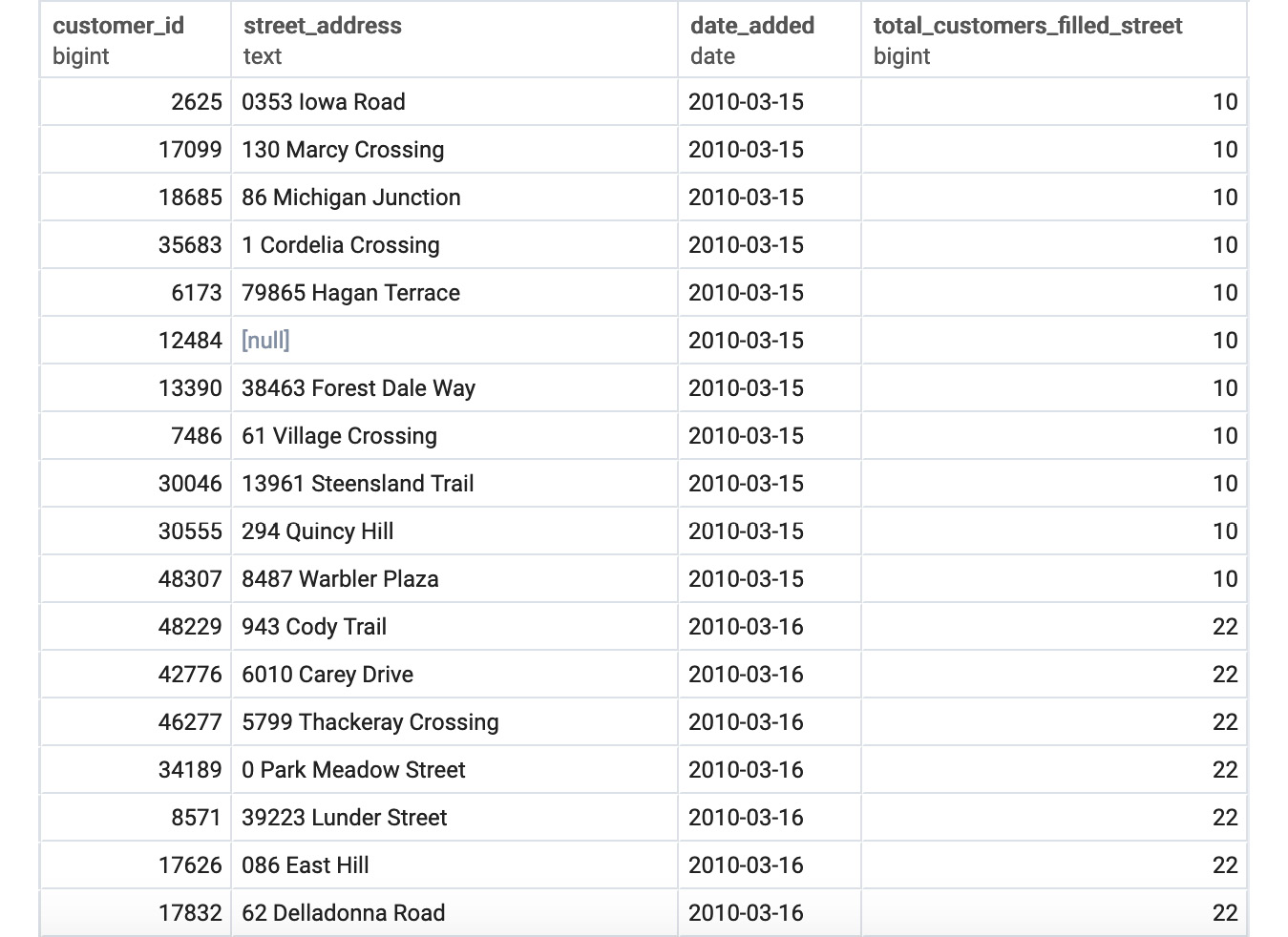
Figure 5.8: Street address filter ordered by the date_added window query

We now have every customer ordered by signup date and can see how the number of people filling out the street field changes over time.

In this exercise, we have learned how to use window functions to analyze data.

The WINDOW Keyword

Now that we understand the basics of window functions, we will introduce some syntax that will make it easier to write window functions. For some queries, you may be interested in calculating the exact same window for different functions. For example, you may be interested in calculating a running total number of customers and the number of customers with a title in each gender with the following query:

SELECT customer_id, title, first_name, last_name, gender,

COUNT(*) OVER (PARTITION BY gender ORDER BY customer_id) as total_customers,

SUM(CASE WHEN title IS NOT NULL THEN 1 ELSE 0 END)

    OVER (PARTITION BY gender ORDER BY customer_id) as total_customers_title

FROM customers

ORDER BY customer_id;

The following is the output of the preceding code:

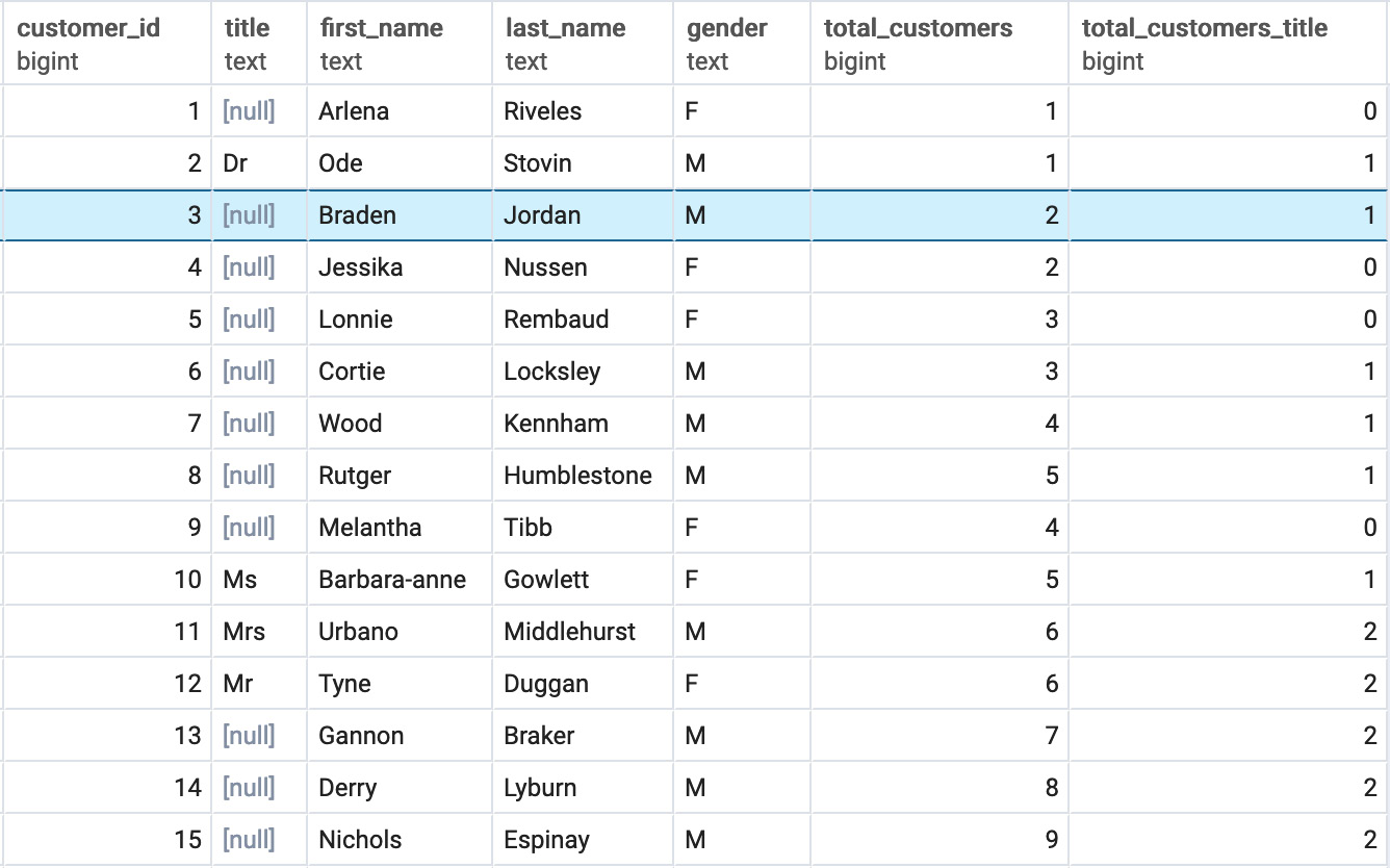
Figure 5.9: Running total of customers overall and with the title by gender window query

Although the query gives you the result, it can be tedious to write, especially the WINDOW clause. Is there a way in which we can simplify it? The answer is yes, and that is with another WINDOW clause. The WINDOW clause facilitates the aliasing of a window.

With our previous query, we can simplify the query by writing it as follows:

SELECT customer_id, title, first_name, last_name, gender,

COUNT(*) OVER w as total_customers,

SUM(CASE WHEN title IS NOT NULL THEN 1 ELSE 0 END)

    OVER w as total_customers_title

FROM customers

WINDOW w AS (PARTITION BY gender ORDER BY customer_id)

ORDER BY customer_id;

This query should give you the same result as seen in Figure 5.9. However, we did not have to write a long PARTITION BY and ORDER BY query for each window function. Instead, we simply made an alias with the defined window w.

Statistics with Window Functions

Now that we understand how window functions work, we can start using them to calculate useful statistics, such as ranks, percentiles, and rolling statistics.

In the following table, we have summarized a variety of statistical functions that are useful. It is also important to emphasize again that all aggregate functions can also be used as window functions (AVG, SUM, COUNT, and so on):

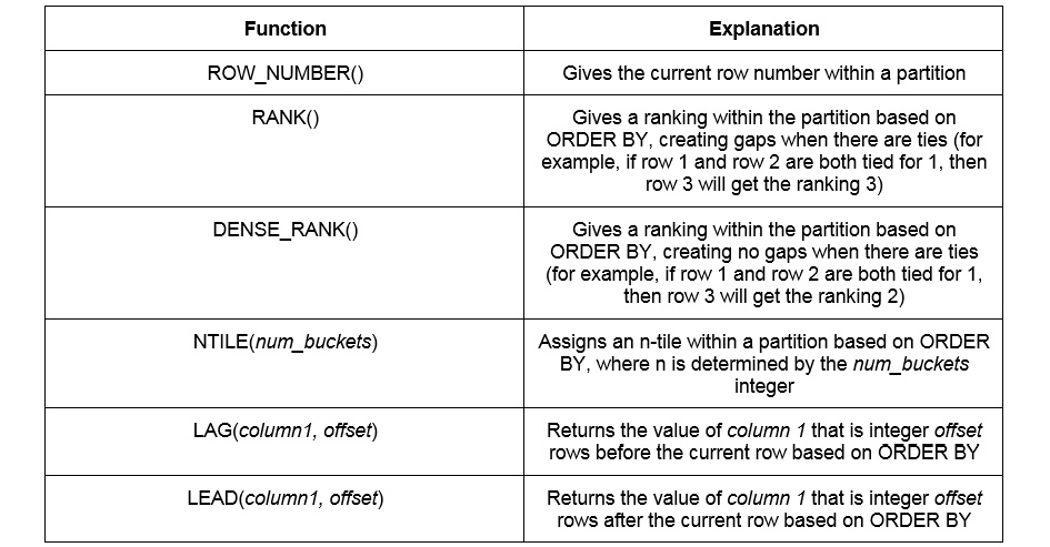
Figure 5.10: Statistical window functions

Exercise 17: Rank Order of Hiring

ZoomZoom would like to promote salespeople at their regional dealerships to management and would like to consider tenure in their decision. Write a query that will rank the order of users according to their hire date for each dealership:

1. Open your favorite SQL client and connect to the sqlda database.
2. Calculate a rank for every salesperson, with a rank of 1 going to the first hire, 2 to the second hire, and so on, using the RANK() function:

   SELECT *,

   RANK() OVER (PARTITION BY dealership_id ORDER BY hire_date)

   FROM salespeople

   WHERE termination_date IS NULL;

   The following is the output of the preceding code:

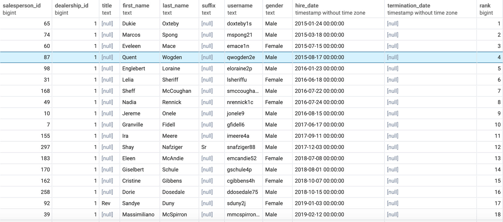
Figure 5.11: Salespeople rank-ordered by tenure

Here, you can see every salesperson with their info and rank in the rank column based on their hire date for each dealership.

In this exercise, we use the RANK() function to rank the data in a dataset in a certain order.

Note

DENSE_RANK() could also just be used as easily as RANK().

Window Frame

When we discussed the basics of window functions, it was mentioned that, by default, a window is set for each row to encompass all rows from the first row in the partition to the current row, as seen in Figure 5.5. However, this is the default and can be adjusted using the window frame clause. A windows function query using the window frame clause would look like the following:

SELECT {columns},

{window_func} OVER (PARTITION BY {partition_key} ORDER BY {order_key} {rangeorrows} BETWEEN {frame_start} AND {frame_end})

FROM {table1};

Here, {columns} are the columns to retrieve from tables for the query, {window_func} is the window function you want to use, {partition_key} is the column or columns you want to partition on (more on this later), {order_key} is the column or columns you want to order by, {rangeorrows} is either the keyword RANGE or the keyword ROWS, {frame_start} is a keyword indicating where to start the window frame, {frame_end} is a keyword indicating where to end the window frame, and {table1} is the table or joined tables you want to pull data from.

One point of difference to consider is the difference between using RANGE or ROW in a frame clause. ROW refer to actual rows and will take the rows before and after the current row to calculate values. RANGE differs when two rows have the same values based on the ORDER BY clause used in the window. If the current row used in the window calculation has the same value in the ORDER BY clause as one or more rows, then all of these rows will be added to the window frame.

Another point is to consider the values that {frame_start} and {frame_end} can take. To give further details, {frame_start} and {frame_end} can be one of the following values:

• UNBOUNDED PRECEDING: a keyword that, when used for {frame_start}, refers to the first record of the partition, and, when used for {frame_end}, refers to the last record of the partition
• {offset} PRECEDING: a keyword referring to integer {offset} rows or ranges before the current row
• CURRENT ROW: the current row
• {offset} FOLLOWING: a keyword referring to integer {offset} rows or ranges after the current row

By adjusting the window, various useful statistics can be calculated. One such useful statistic is the rolling average. The rolling average is simply the average for a statistic in a given time window. Let's say you want to calculate the 7-day rolling average of sales over time for ZoomZoom. This calculation could be accomplished with the following query:

WITH daily_sales as (

SELECT sales_transaction_date::DATE,

SUM(sales_amount) as total_sales

FROM sales

GROUP BY 1

),

moving_average_calculation_7 AS (

SELECT sales_transaction_date, total_sales,

AVG(total_sales) OVER (ORDER BY sales_transaction_date ROWS BETWEEN 7 PRECEDING and CURRENT ROW) AS sales_moving_average_7,

ROW_NUMBER() OVER (ORDER BY sales_transaction_date) as row_number

FROM daily_sales

ORDER BY 1)

SELECT sales_transaction_date,

CASE WHEN row_number>=7 THEN sales_moving_average_7 ELSE NULL END

   AS sales_moving_average_7

FROM moving_average_calculation_7;

The following is the output of the preceding code:

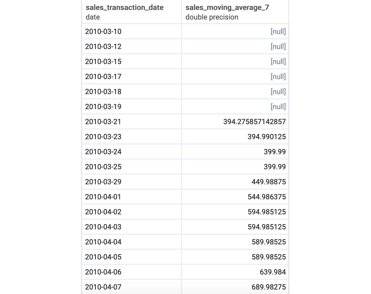
Figure 5.12: The 7-day moving average of sales

The reason the first 7 rows are null is that the 7-day moving average is only defined if there are 7 days' worth of information, and the window calculation will still calculate values for the first 7 days using the first few days.

Exercise 18: Team Lunch Motivation

To help improve sales performance, the sales team has decided to buy lunch for all salespeople at the company every time they beat the figure for best daily total earnings achieved over the last 30 days. Write a query that produces the total sales in dollars for a given day and the target the salespeople have to beat for that day, starting from January 1, 2019:

1. Open your favorite SQL client and connect to the sqlda database.
2. Calculate the total sales for a given day and the target using the following query:

   WITH daily_sales as (

   SELECT sales_transaction_date::DATE,

   SUM(sales_amount) as total_sales

   FROM sales

   GROUP BY 1

   ),

   sales_stats_30 AS (

   SELECT sales_transaction_date, total_sales,

   MAX(total_sales) OVER (ORDER BY sales_transaction_date ROWS BETWEEN 30 PRECEDING and 1 PRECEDING)

   AS max_sales_30

   FROM daily_sales

   ORDER BY 1)

   SELECT sales_transaction_date,

   total_sales,

   max_sales_30

   FROM sales_stats_30

   WHERE sales_transaction_date>='2019-01-01';

   You should get the following results:

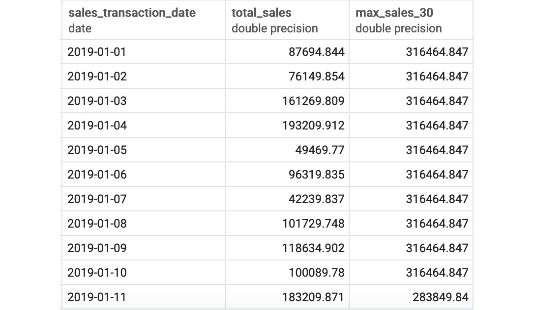
Figure 5.13: Best sales over the last 30 days

Notice the use of a window frame from 30 PRECEDING to 1 PRECEDING to remove the current row from the calculation.

As can be seen in this exercise, window frames make calculating moving statistics simple, and even kind of fun!

Activity 7: Analyzing Sales Using Window Frames and Window Functions

It's the holidays, and it's time to give out Christmas bonuses at ZoomZoom. Sales team want to see how the company has performed overall, as well as how individual dealerships have performed within the company. To achieve this, ZoomZoom's head of Sales would like you to run an analysis for them:

1. Open your favorite SQL client and connect to the sqlda database.
2. Calculate the total sales amount by day for all of the days in the year 2018 (that is, before the date January 1, 2019).
3. Calculate the rolling 30-day average for the daily number of sales deals.
4. Calculate what decile each dealership would be in compared to other dealerships based on their total sales amount.

Expected Output:

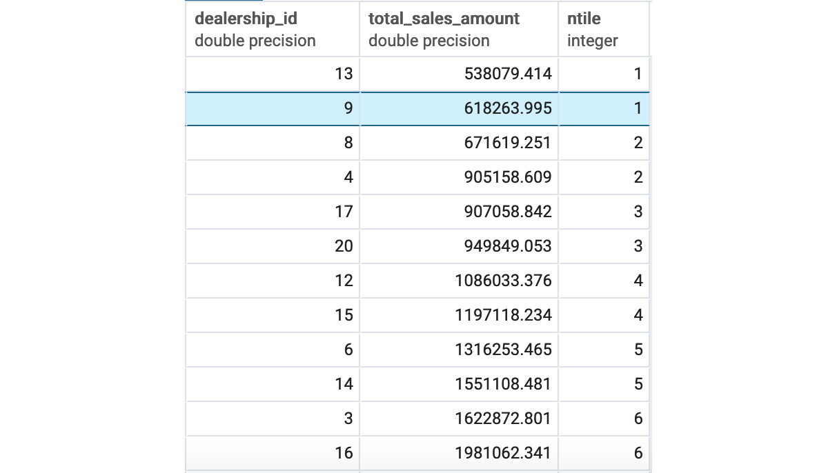
Figure 5.14: Decile for dealership sales amount

Note

The solution for the activity can be found on page 325.

Summary

In this chapter, we learned about the power of window functions. We looked at how to construct a basic window function using OVER, PARTITION BY, and ORDER BY. We then looked at how to calculate statistics using window functions, and how to adjust a window frame to calculate rolling statistics.

In the next chapter, we will look at how to import and export data in order to utilize SQL with other programs. We will use the COPY command to upload data to your database in bulk. We will also use Excel to process data from your database and then simplify your code using SQLAlchemy.