Appendix

About

This section is included to assist the readers to perform the activities in the book. It includes detailed steps that are to be performed by the readers to achieve the objectives of the activities.

Chapter 1: Understanding and Describing Data

Activity 1: Classifying a New Dataset

Solution

1. The unit of observation is a car purchase.
2. Date and Sales Amount are quantitative, while Make is qualitative.
3. While there could be many ways to convert Make into quantitative data, one commonly accepted method would be to map each of the Make types to a number. For instance, Ford could map to 1, Honda could map to 2, Mazda could map to 3, Toyota could map to 4, Mercedes could map to 5, and Chevy could map to 6.

Activity 2: Exploring Dealership Sales Data

Solution

1. Open Microsoft Excel to a blank workbook.
2. Go to the Data tab and click on From Text.
3. Find the path to the dealerships.csv file and click on OK.
4. Choose the Delimited option in the Text Import Wizard dialog box, and make sure to start the import at row 1. Now, click on Next.
5. Select the delimiter for your file. As this file is only one column, it has no delimiters, although CSVs traditionally use commas as delimiters (in future, use whatever is appropriate for your dataset). Now, click on Next.
6. Select General for the Column Data Format. Now, click on Finish.
7. For the dialog box asking Where you want to put the data?, select Existing Sheet, and leave what is in the textbox next to it as is. Now, click on OK. You should see something similar to the following diagram:
   

   Figure 1.33: The dealerships.csv file loaded

8. Histograms may vary a little bit depending on what parameters are chosen, but it should look similar to the following:
   

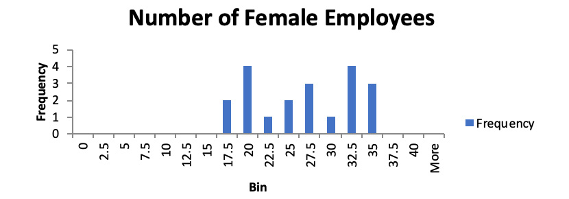
   Figure 1.34: A histogram showing the number of female employees

9. Here, the mean sales are $171,603,750.13, and the median sales are $184,939,292.
10. The standard deviation of sales is $50,152,290.42.
11. The Boston, MA dealership is an outlier. This can be shown graphically or by using the IQR method.
12. You should get the following four quintiles:
13. 

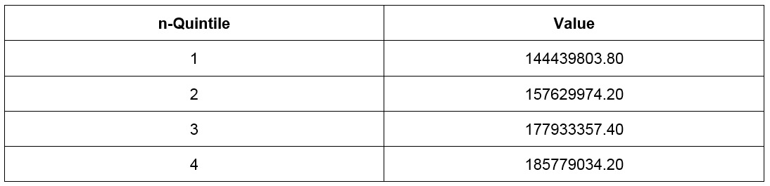
    Figure 1.35: Quintiles and their values

14. Removing the outlier of Boston, you should get a correlation coefficient of 0.55. This value implies that there is a strong correlation between the number of female employees and the sales of a dealership. While this may be evidence that more female employees lead to more revenue, it may also be a simple consequence of a third effect. In this case, larger dealerships have a larger number of employees in general, which also means that women will be at these locations as well. There may be other correlational interpretations as well.

Chapter 2: The Basics of SQL for Analytics

Activity 3: Querying the customers Table Using Basic Keywords in a SELECT Query

Solution

1. Open your favorite SQL client and connect to the sqlda database. Examine the schema for the customers table from the schema dropdown. Notice the names of the columns, the same as we did in Exercise 6, Querying Salespeople, for the salespeople table.
2. Execute the following query to fetch customers in the state of Florida in alphabetical order:

   SELECT email

   FROM customers

   WHERE state='FL'

   ORDER BY email

   The following is the output of the preceding code:

   

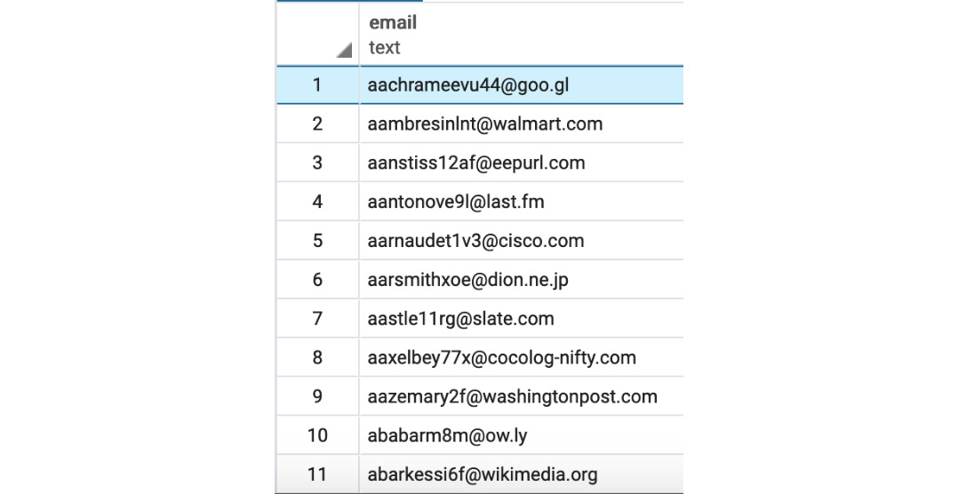
   Figure 2.13: Emails of customers from Florida in alphabetical order

3. Execute the following query to pull all the first names, last names, and email addresses for ZoomZoom customers in New York City in the state of New York. The customers would be ordered alphabetically by the last name followed by the first name:

   SELECT first_name, last_name, email

   FROM customers

   WHERE city='New York City'

   and state='NY'

   ORDER BY last_name, first_name

   The following is the output of the preceding code:

   

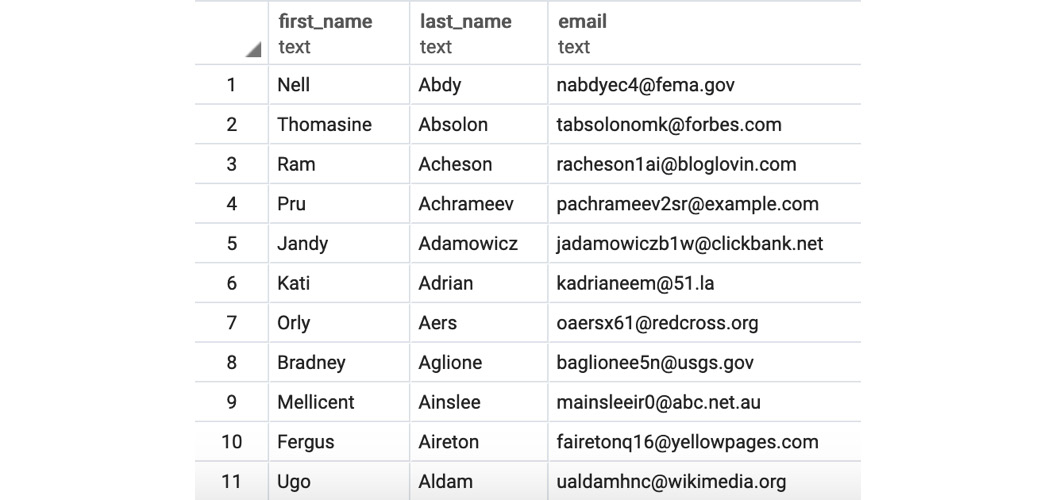
   Figure 2.14: Details of customers from New York City in alphabetical order

4. Execute the following query to fetch all customers that have a phone number ordered by the date the customer was added to the database:

   SELECT *

   FROM customers

   WHERE phone IS NOT NULL

   ORDER BY date_added

   The following is the output of the preceding code:

   

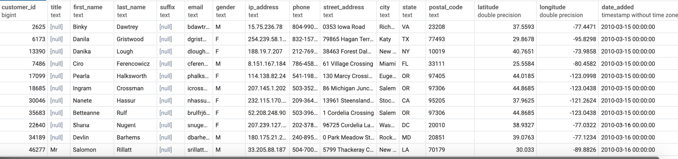
Figure 2.15: Customers with a phone number ordered by the date the customer was added to the database

Activity 4: Marketing Operations

Solution

1. Open your favorite SQL client and connect to the sqlda database.
2. Run the following query to create the table with New York City customers:

   CREATE TABLE customers_nyc AS (

   SELECT * FROM

   customers

   where city='New York City'

   and state='NY');

   

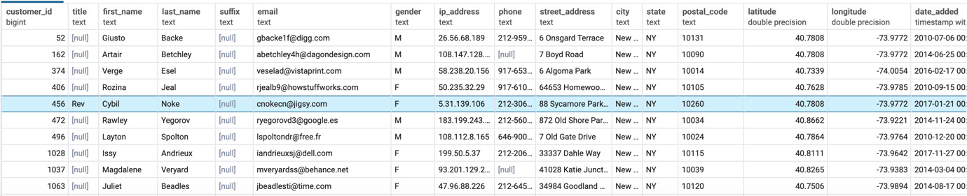
   Figure 2.16: Table showing customers from New York City

3. Then, run the following query statement to delete users with the postal code 10014:

   DELETE FROM customers_nyc WHERE postal_code='10014';

4. Execute the following query to add the new event column:

   ALTER TABLE customers_nyc ADD COLUMN event text;

5. Update the customers_nyc table and set the event to thank-you party using the following query:

   UPDATE customers_nyc

   SET event = 'thank-you party';

   

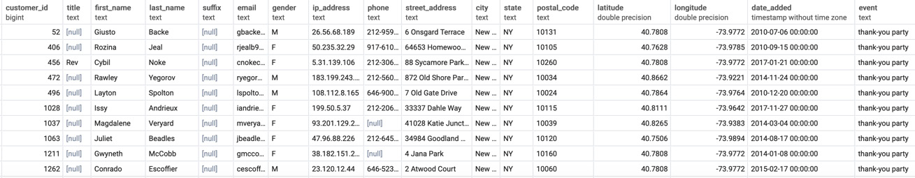
   Figure 2.17: The customers_nyc table with event set as 'thank-you party'

6. Now, we will delete the customers_nyc table as asked by the manager using DROP TABLE:

   DROP TABLE customers_nyc;

   This will delete the customers_nyc table from the database.

Chapter 3: SQL for Data Preparation

Activity 5: Building a Sales Model Using SQL Techniques

Solution

1. Open your favorite SQL client and connect to the sqlda database.
2. Follow the steps mentioned with the scenario and write the query for it. There are many approaches to this query, but one of these approaches could be:

   SELECT

   c.*,

   p.*,

   COALESCE(s.dealership_id, -1),

   CASE WHEN p.base_msrp - s.sales_amount >500 THEN 1 ELSE 0 END AS high_savings

   FROM sales s

   INNER JOIN customers c ON c.customer_id=s.customer_id

   INNER JOIN products p ON p.product_id=s.product_id

   LEFT JOIN dealerships d ON s.dealership_id = d.dealership_id;

3. The following is the output of the preceding code:

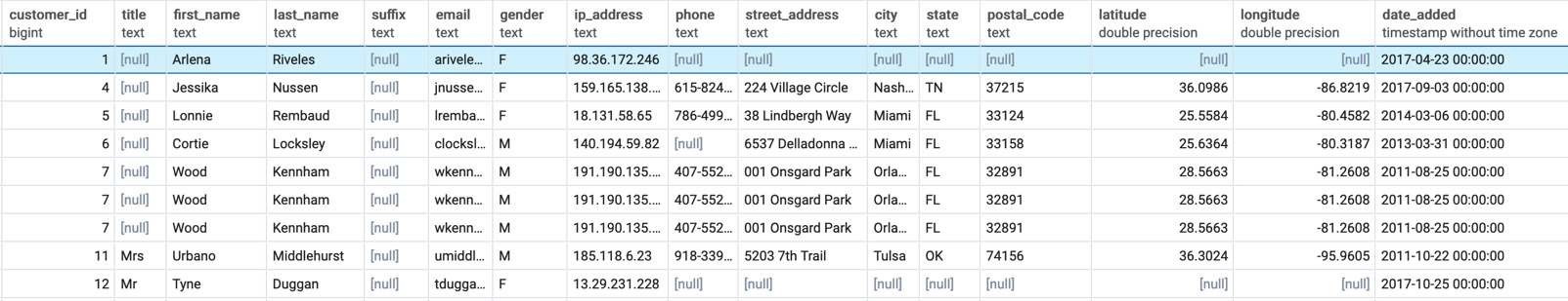
Figure 3.21: Building a sales model query

Thus, have the data to build a new model that will help the data science team to predict which customers are the best prospects for remarketing from the output generated.

Chapter 4: Aggregate Functions for Data Analysis

Activity 6: Analyzing Sales Data Using Aggregate Functions

Solution

1. Open your favorite SQL client and connect to the sqlda database.
2. Calculate the number of unit sales the company has achieved by using the COUNT function:

   SELECT COUNT(*)

   FROM sales;

   You should get 37,711 sales.

3. Determine the total sales amount in dollars for each state; we can use the SUM aggregate function here:

   SELECT c.state, SUM(sales_amount) as total_sales_amount

   FROM sales s

   INNER JOIN customers c ON c.customer_id=s.customer_id

   GROUP BY 1

   ORDER BY 1;

   You will get the following output:

   

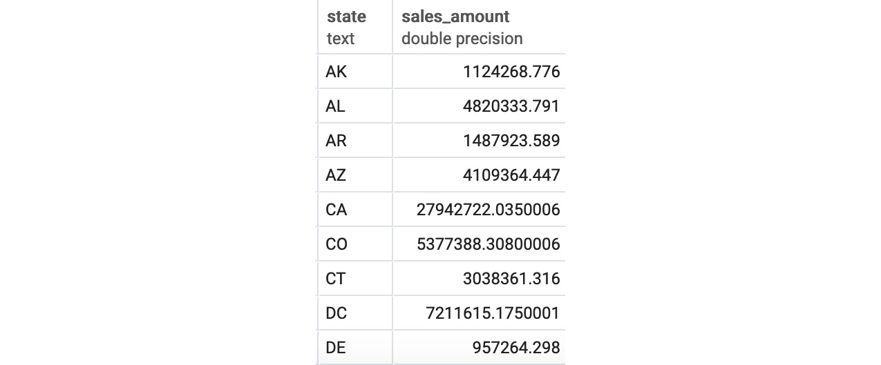
   Figure 4.23: Total sales in dollars by US state

4. Determine the top five dealerships in terms of most units sold, using the GROUP BY clause and set LIMIT as 5:

   SELECT s.dealership_id, COUNT(*)

   FROM sales s

   WHERE channel='dealership'

   GROUP BY 1

   ORDER BY 2 DESC

   LIMIT 5

   You should get the following output:

   

   Figure 4.24: Top five dealerships by units sold

5. Calculate the average sales amount for each channel, as seen in the sales table, and look at the average sales amount first by channel sales, then by product_id, and then by both together. This can be done using GROUPING SETS as follows:

   SELECT s.channel, s.product_id, AVG(sales_amount) as avg_sales_amount

   FROM sales s

   GROUP BY

   GROUPING SETS(

   (s.channel), (s.product_id),

   (s.channel, s.product_id)

   )

   ORDER BY 1, 2

   You should get the following output:

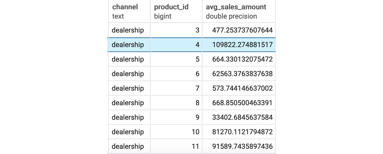
Figure 4.25: Sales after the GROUPING SETS channel and product_id

From the preceding figure, we can see the channel and product ID of all the products as well as the sales amount generated by each product.

Using aggregates, you have unlocked patterns that will help your company understand how to make more revenue and make the company better overall.

Chapter 5: Window Functions for Data Analysis

Activity 7: Analyzing Sales Using Window Frames and Window Functions

Solution

1. Open your favorite SQL client and connect to the sqlda database.
2. Calculate the total sales amount for all individual months in 2018 using the SUM function:

   SELECT sales_transaction_date::DATE,

   SUM(sales_amount) as total_sales_amount

   FROM sales

   WHERE sales_transaction_date>='2018-01-01'

   AND sales_transaction_date<'2019-01-01'

   GROUP BY 1

   ORDER BY 1;

   The following is the output of the preceding code:

   

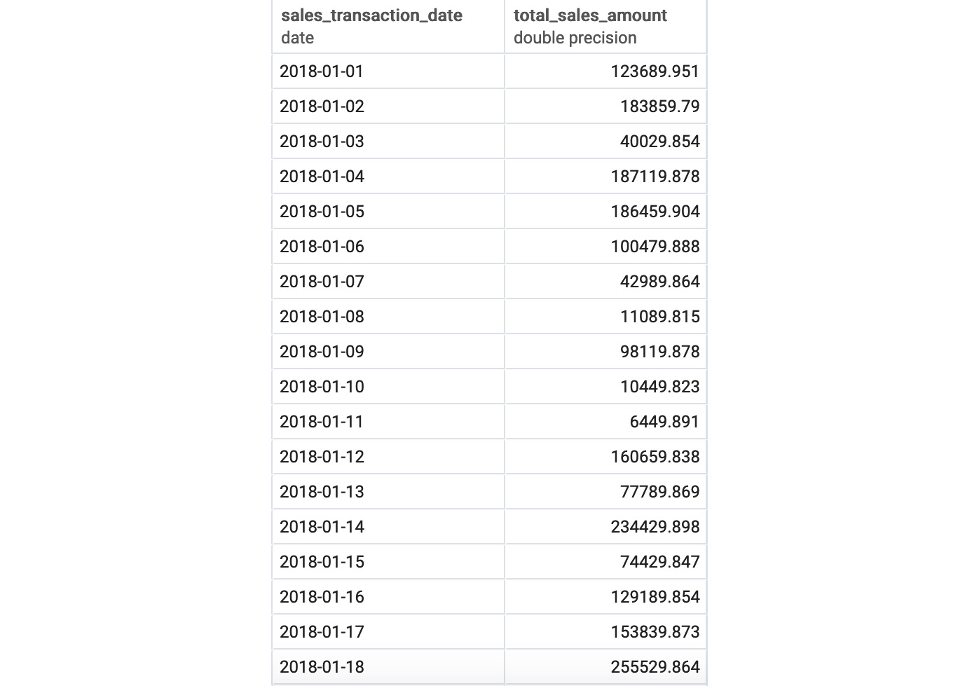
   Figure 5.15: Total sales amount by month

3. Now, calculate the rolling 30-day average for the daily number of sales deals, using a window frame:

   WITH daily_deals as (

   SELECT sales_transaction_date::DATE,

   COUNT(*) as total_deals

   FROM sales

   GROUP BY 1

   ),

   moving_average_calculation_30 AS (

   SELECT sales_transaction_date, total_deals,

   AVG(total_deals) OVER (ORDER BY sales_transaction_date ROWS BETWEEN 30 PRECEDING and CURRENT ROW) AS deals_moving_average,

   ROW_NUMBER() OVER (ORDER BY sales_transaction_date) as row_number

   FROM daily_deals

   ORDER BY 1)

   SELECT sales_transaction_date,

   CASE WHEN row_number>=30 THEN deals_moving_average ELSE NULL END

      AS deals_moving_average_30

   FROM moving_average_calculation_30

   WHERE sales_transaction_date>='2018-01-01'

   AND sales_transaction_date<'2019-01-01';

   The following is the output of the preceding code:

   

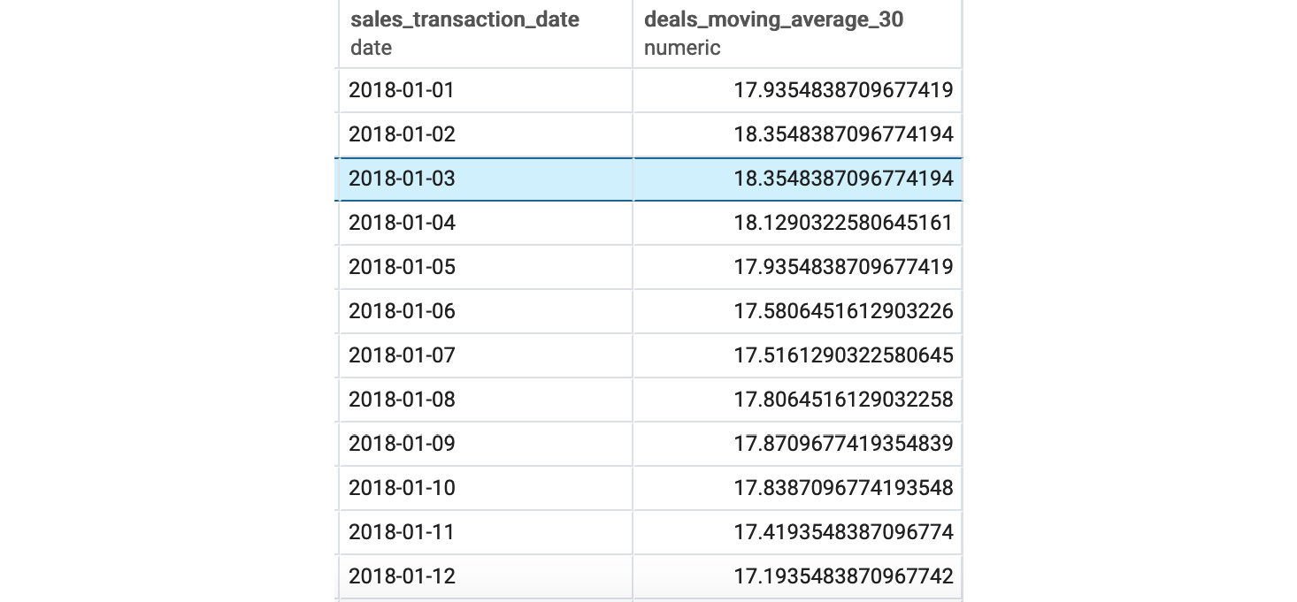
   Figure 5.16: Rolling 30-day average of sales

4. Next, calculate what decile each dealership would be in compared to other dealerships based on the total sales amount, using window functions:

   WITH total_dealership_sales AS

   (

   SELECT dealership_id,

   SUM(sales_amount) AS total_sales_amount

   FROM sales

   WHERE sales_transaction_date>='2018-01-01'

   AND sales_transaction_date<'2019-01-01'

   AND channel='dealership'

   GROUP BY 1

   )

   SELECT *,

   NTILE(10) OVER (ORDER BY total_sales_amount)

   FROM total_dealership_sales;

   The following is the output of the preceding code:

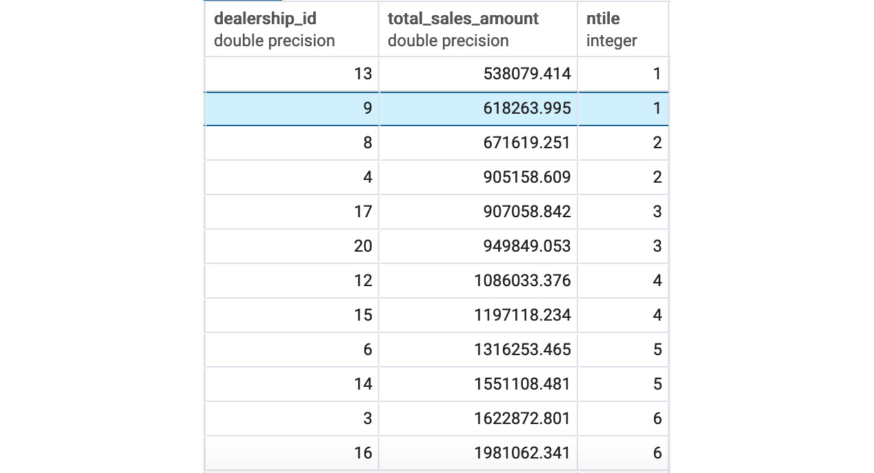
Figure 5.17: Decile for dealership sales amount

Chapter 6: Importing and Exporting Data

Activity 8: Using an External Dataset to Discover Sales Trends

Solution

1. The dataset can be downloaded from GitHub using the link provided. Once you go to the web page, you should be able to Save Page As… using the menus on your browser:
   

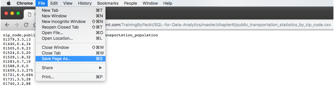
   Figure 6.24: Saving the public transportation .csv file

2. The simplest way to transfer the data in a CSV file to pandas is to create a new Jupyter notebook. At the command line, type jupyter notebook (if you do not have a notebook server running already). In the browser window that pops up, create a new Python 3 notebook. In the first cell, you can type in the standard import statements and the connection information (replacing your_X with the appropriate parameter for your database connection):

   from sqlalchemy import create_engine

   import pandas as pd

   % matplotlib inline

   cnxn_string = ("postgresql+psycopg2://{username}:{pswd}"

                  "@{host}:{port}/{database}")

   engine = create_engine(cnxn_string.format(

       username="your_username",

       pswd="your_password",

       host="your_host",

       port=5432,

       database="your_db"))

3. We can read in the data using a command such as the following (replacing the path specified with the path to the file on your local computer):

   data = pd.read_csv("~/Downloads/public_transportation'_statistics_by_zip_code.csv", dtype={'zip_code':str})

   Check that the data looks correct by creating a new cell, entering data, and then hitting Shift + Enter to see the contents of data. You can also use data.head() to see just the first few rows:

   

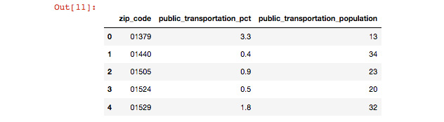
   Figure 6.25: Reading the public transportation data into pandas

4. Now, we can transfer data to our database using data.to_sql():

   import csv

   from io import StringIO

   def psql_insert_copy(table, conn, keys, data_iter):

       # gets a DBAPI connection that can provide a cursor

       dbapi_conn = conn.connection

       with dbapi_conn.cursor() as cur:

           s_buf = StringIO()

           writer = csv.writer(s_buf)

           writer.writerows(data_iter)

           s_buf.seek(0)

           columns = ', '.join('"{}"'.format(k) for k in keys)

           if table.schema:

               table_name = '{}.{}'.format(table.schema, table.name)

           else:

               table_name = table.name

           sql = 'COPY {} ({}) FROM STDIN WITH CSV'.format(

               table_name, columns)

           cur.copy_expert(sql=sql, file=s_buf)

   data.to_sql('public_transportation_by_zip', engine, if_exists='replace', method=psql_insert_copy)

5. Looking at the maximum and minimum values, we do see something strange: the minimum value is -666666666. We can assume that these values are missing, and we can remove them from the dataset:

   SELECT

       MAX(public_transportation_pct) AS max_pct,

       MIN(public_transportation_pct) AS min_pct

   FROM public_transportation_by_zip;

   

   Figure 6.26: Screenshot showing minimum and maximum values

6. In order to calculate the requested sales amounts, we can run a query in our database. Note that we will have to filter out the erroneous percentages below 0 based on our analysis in step 6. There are several ways to do this, but this single statement would work:

   SELECT

       (public_transportation_pct > 10) AS is_high_public_transport,

       COUNT(s.customer_id) * 1.0 / COUNT(DISTINCT c.customer_id) AS sales_per_customer

   FROM customers c

   INNER JOIN public_transportation_by_zip t ON t.zip_code = c.postal_code

   LEFT JOIN sales s ON s.customer_id = c.customer_id

   WHERE public_transportation_pct >= 0

   GROUP BY 1

   ;

   Here's an explanation of this query:

   We can identify customers living in an area with public transportation by looking at the public transportation data associated with their postal code. If public_transportation_pct > 10, then the customer is in a high public transportation area. We can group by this expression to identify the population that is or is not in a high public transportation area.

   We can look at sales per customer by counting the sales (for example, using the COUNT(s.customer_id) aggregate) and dividing by the unique number of customers (for example, using the COUNT(DISTINCT c.customer_id) aggregate). We want to make sure that we retain fractional values, so we can multiply by 1.0 to cast the entire expression to a float: COUNT(s.customer_id) * 1.0 / COUNT(DISTINCT c.customer_id).

   In order to do this, we need to join our customer data to the public transportation data, and finally to the sales data. We need to exclude all zip codes where public_transportation_pct is greater than, or equal to, 0 so that we exclude the missing data (denoted by -666666666).

   Finally, we end with the following query:

   

   Figure 6.27: Calculating the requested sales amount

   From this, we see that customers in high public transportation areas have 12% more product purchases than customers in low public transportation areas.

7. If we try to plot our data, we will get a strange distribution with two bars. This is because of the outlier values that we discovered in step 5. Instead, we can read this data from our database, and add a WHERE clause to remove the outlier values:

   data = pd.read_sql_query('SELECT * FROM public_transportation_by_zip WHERE public_transportation_pct > 0 AND public_transportation_pct < 50', engine)

   data.plot.hist(y='public_transportation_pct')

   

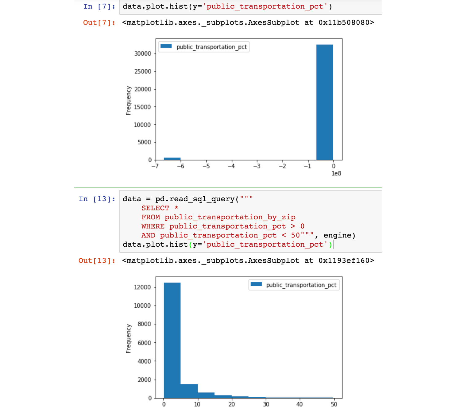
   Figure 6.28: Jupyter notebook with analysis of the public transportation data

8. We can then rerun our command from step 5 to get the timing of the standard to_sql() function:

   data.to_sql('public_transportation_by_zip', engine, if_exists='replace')

   

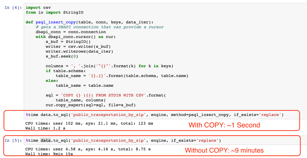
   Figure 6.29: Inserting records with COPY and without COPY is much faster

9. For this analysis, we can actually tweak the query from step 7:

   CREATE TEMP VIEW public_transport_statistics AS (

       SELECT

           10 * ROUND(public_transportation_pct/10) AS public_transport,

           COUNT(s.customer_id) * 1.0 / COUNT(DISTINCT c.customer_id) AS sales_per_customer

       FROM customers c

       INNER JOIN public_transportation_by_zip t ON t.zip_code = c.postal_code

       LEFT JOIN sales s ON s.customer_id = c.customer_id

       WHERE public_transportation_pct >= 0

       GROUP BY 1

   );

   copy (SELECT * FROM public_transport_statistics) TO 'public_transport_distribution.csv' CSV HEADER;

   First, we want to wrap our query in a temporary view, public_transport_statistics, so that we easily write the result to a CSV file later.

   Next is the tricky part: we want to aggregate the public transportation statistics somehow. What we can do is round this percentage to the nearest 10%, so 22% would become 20%, and 39% would become 40%. We can do this by dividing the percentage number (represented as 0.0-100.0) by 10, rounding off, and then multiplying back by 10: 10 * ROUND(public_transportation_pct/10).

   The logic for the remainder of the query is explained in step 6.

10. Next, we open up the public_transport_distribution.csv file in Excel:

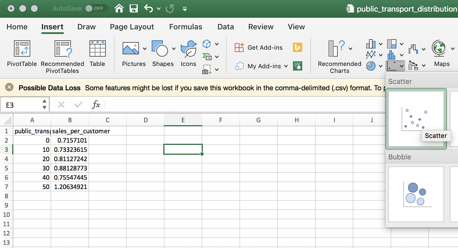
Figure 6.30: Excel workbook containing the data from our query

After creating the scatterplot, we get the following result, which shows a clear positive relationship between public transportation and sales in the geographical area:

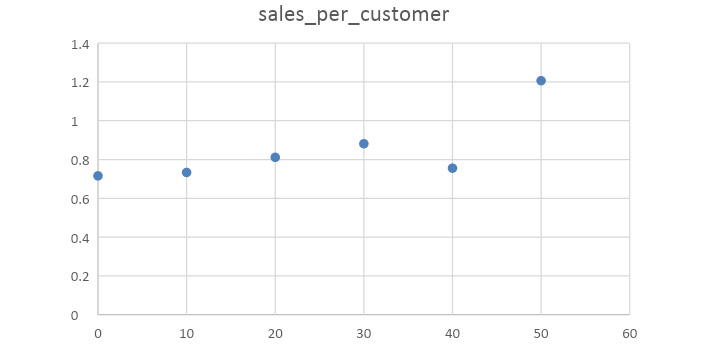
Figure 6.31: Sales per customer versus public transportation percentage

Based on all this analysis, we can say that there is a positive relationship between geographies with public transportation and demand for electric vehicles. Intuitively, this makes sense, because electric vehicles could provide an alternative transportation option to public transport for getting around cities. As a result of this analysis, we would recommend that ZoomZoom management should consider expanding in regions with high public transportation and urban areas.

Chapter 7: Analytics Using Complex Data Types

Activity 9: Sales Search and Analysis

Solution

1. First, create the materialized view on the customer_sales table:

   CREATE MATERIALIZED VIEW customer_search AS (

       SELECT

           customer_json -> 'customer_id' AS customer_id,

           customer_json,

           to_tsvector('english', customer_json) AS search_vector

       FROM customer_sales

   );

2. Create the GIN index on the view:

   CREATE INDEX customer_search_gin_idx ON customer_search USING GIN(search_vector);

3. We can solve the request by using our new searchable database:

   SELECT

       customer_id,

       customer_json

   FROM customer_search

   WHERE search_vector @@ plainto_tsquery('english', 'Danny Bat');

   This results in eight matching rows:

   

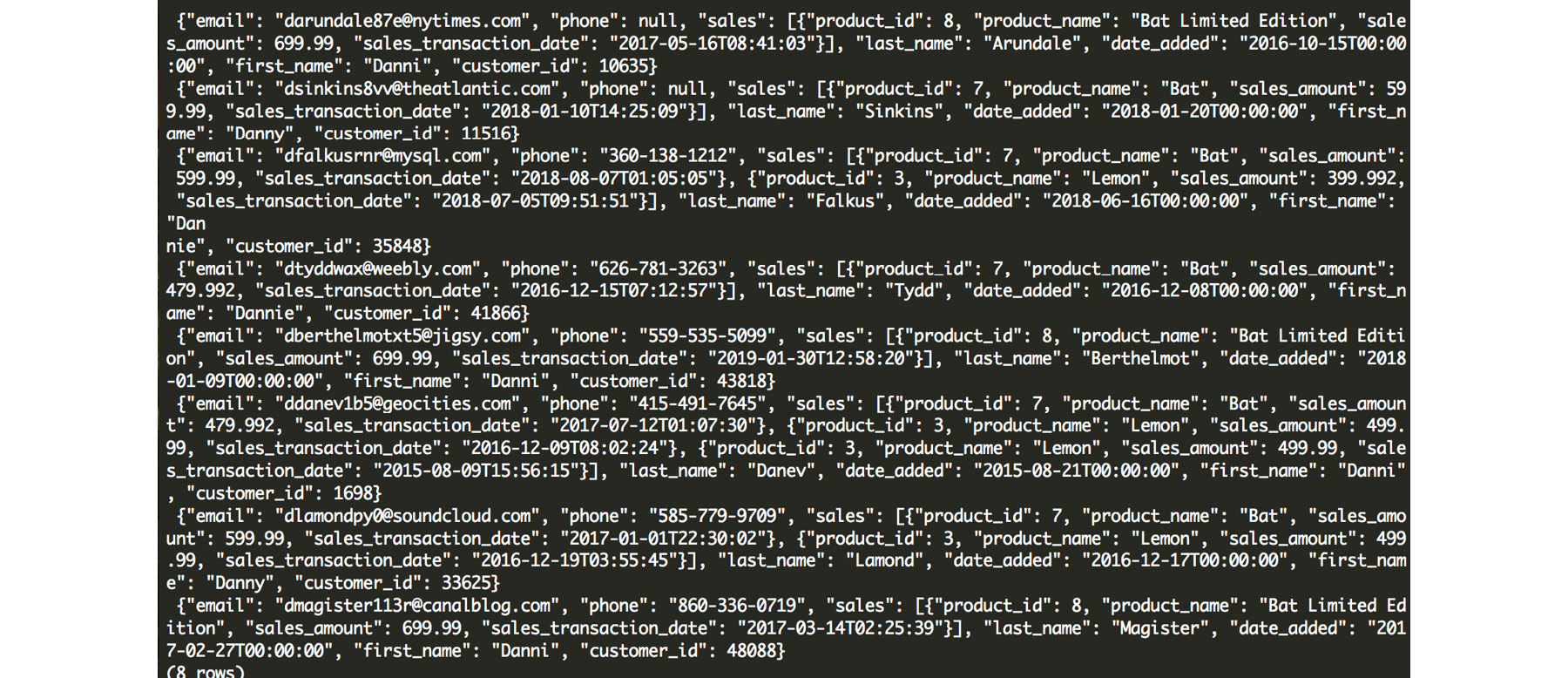
   Figure 7.29: Resulting matches for our "Danny Bat" query

   In this complex task, we need to find customers who match with both a scooter and an automobile. That means we need to perform a query for each combination of scooter and automobile.

4. We need to produce the unique list of scooters and automobiles (and remove limited editions releases) using DISTINCT:

   SELECT DISTINCT

       p1.model,

       p2.model

   FROM products p1

   LEFT JOIN products p2 ON TRUE

   WHERE p1.product_type = 'scooter'

   AND p2.product_type = 'automobile'

   AND p1.model NOT ILIKE '%Limited Edition%';

   This produces the following output:

   

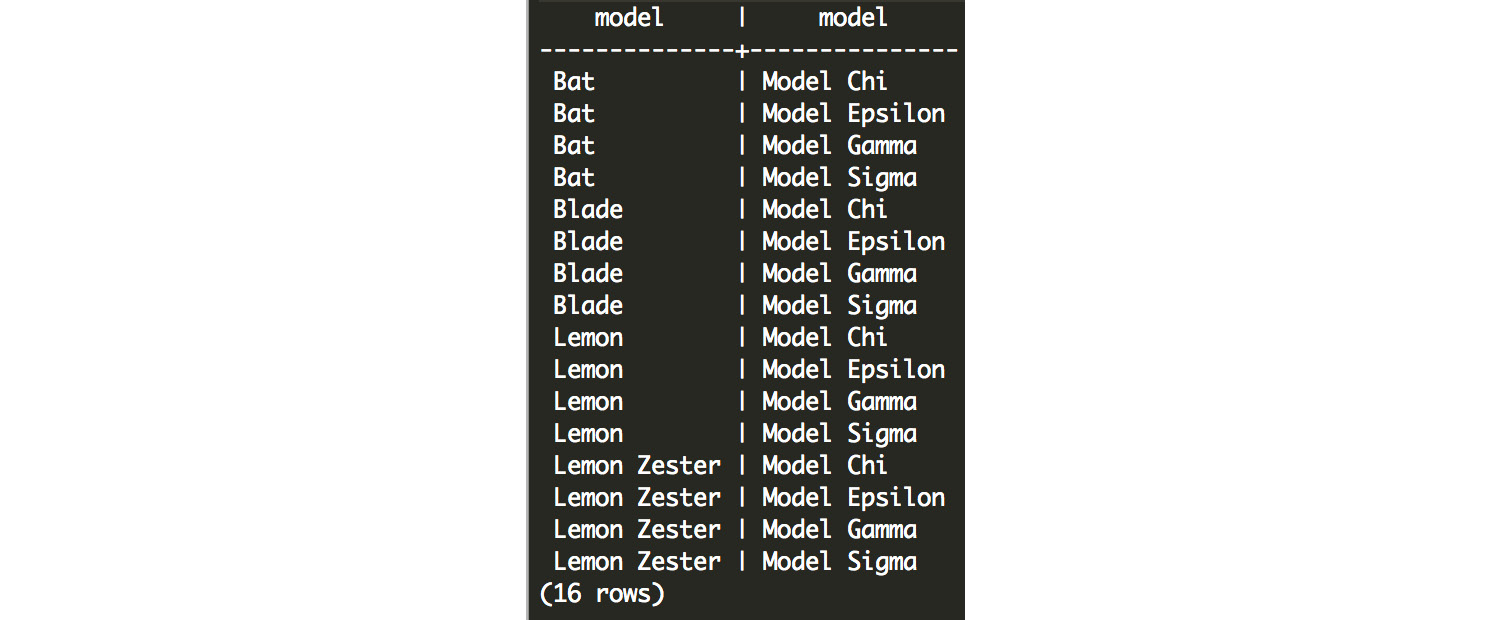
   Figure 7.30: All combinations of scooters and automobiles

5. Next, we need to transform the output into the query:

   SELECT DISTINCT

       plainto_tsquery('english', p1.model) &&

       plainto_tsquery('english', p2.model)

   FROM products p1

   LEFT JOIN products p2 ON TRUE

   WHERE p1.product_type = 'scooter'

   AND p2.product_type = 'automobile'

   AND p1.model NOT ILIKE '%Limited Edition%';

   This produces the following result:

   

   Figure 7.31: Queries for each scooter and automobile combination

6. Query our database using each of these tsquery objects, and count the occurrences for each object:

   SELECT

       sub.query,

       (

           SELECT COUNT(1)

           FROM customer_search

           WHERE customer_search.search_vector @@ sub.query)

   FROM (

       SELECT DISTINCT

           plainto_tsquery('english', p1.model) &&

           plainto_tsquery('english', p2.model) AS query

       FROM products p1

       LEFT JOIN products p2 ON TRUE

       WHERE p1.product_type = 'scooter'

       AND p2.product_type = 'automobile'

       AND p1.model NOT ILIKE '%Limited Edition%'

   ) sub

   ORDER BY 2 DESC;

   The following is the output of the preceding query:

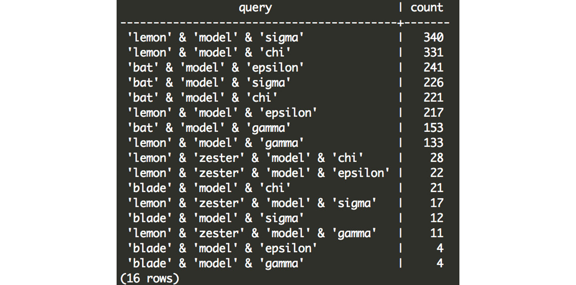
Figure 7.32: Customer counts for each scooter and automobile combination

While there could be a multitude of factors at play here, we see that the lemon scooter and the model sigma automobile is the combination most frequently purchased together, followed by the lemon and model chi. The bat is also fairly frequently purchased with both of those models, as well as the model epsilon. The other combinations are much less common, and it seems that customers rarely purchase the lemon zester, the blade, and the model gamma.

Chapter 8: Performant SQL

Activity 10: Query Planning

Solution:

1. Open PostgreSQL and connect to the sqlda database:

   C:> psql sqlda

2. Use the EXPLAIN command to return the query plan for selecting all available records within the customers table:

   sqlda=# EXPLAIN SELECT * FROM customers;

   This query will produce the following output from the planner:

   

   Figure 8.75: Plan for all records within the customers table

   The setup cost is 0, the total query cost is 1536, the number of rows is 50000, and the width of each row is 140. The cost is actually in cost units, the number of rows is in rows, and the width is in bytes.

3. Repeat the query from step 2 of this activity, this time limiting the number of returned records to 15:

   sqlda=# EXPLAIN SELECT * FROM customers LIMIT 15;

   This query will produce the following output from the planner:

   

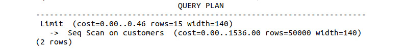
   Figure 8.76: Plan for all records within the customers table with the limit as 15

   Two steps are involved in the query, and the limiting step costs 0.46 units within the plan.

4. Generate the query plan, selecting all rows where customers live within a latitude of 30 and 40 degrees:

   sqlda=# EXPLAIN SELECT * FROM customers WHERE latitude > 30 and latitude < 40;

   This query will produce the following output from the planner:

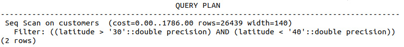
Figure 8.77: Plan for customers living within a latitude of 30 and 40 degrees

The total plan cost is 1786 units, and it returns 26439 rows.

Activity 11: Implementing Index Scans

Solution:

1. Use the EXPLAIN and ANALYZE commands to profile the query plan to search for all records with an IP address of 18.131.58.65:

   EXPLAIN ANALYZE SELECT * FROM customers WHERE ip_address = '18.131.58.65';

   The following output will be displayed:

   

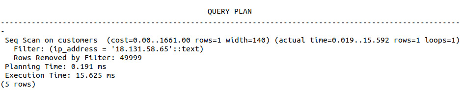
   Figure 8.78: Sequential scan with a filter on ip_address

   The query takes 0.191 ms to plan and 15.625 ms to execute.

2. Create a generic index based on the IP address column:

   CREATE INDEX ON customers(ip_address);

3. Rerun the query of step 1 and note the time it takes to execute:

   EXPLAIN ANALYZE SELECT * FROM customers WHERE ip_address = '18.131.58.65';

   The following is the output of the preceding code:

   

   
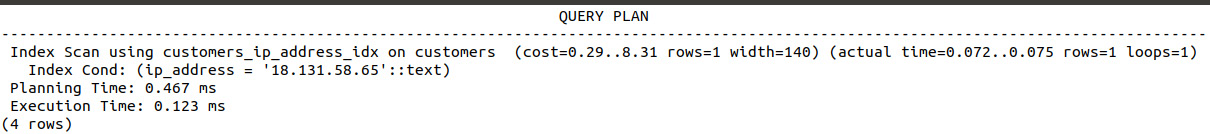
Figure 8.79: Index scan with a filter on ip_address

   The query takes 0.467 ms to plan and 0.123 ms to execute.

4. Create a more detailed index based on the IP address column with the condition that the IP address is 18.131.58.65:

   CREATE INDEX ix_ip_where ON customers(ip_address) WHERE ip_address = '18.131.58.65';

5. Rerun the query of step 1 and note the time it takes to execute.

   EXPLAIN ANALYZE SELECT * FROM customers WHERE ip_address = '18.131.58.65';

   The following is the output of the preceding code:

   

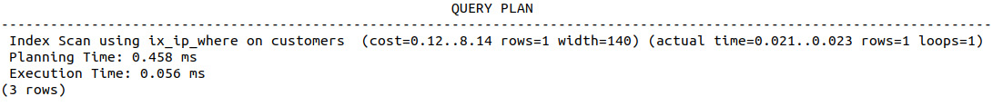
   Figure 8.80: Query plan with reduced execution time due to a more specific index

   The query takes 0.458 ms to plan and 0.056 ms to execute. We can see that both indices took around the same amount of time to plan, with the index that specifies the exact IP address being much faster to execute and slightly quicker to plan as well.

6. Use the EXPLAIN and ANALYZE commands to profile the query plan to search for all records with a suffix of Jr:

   EXPLAIN ANALYZE SELECT * FROM customers WHERE suffix = 'Jr';

   The following output will be displayed:

   

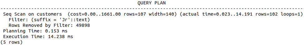
   Figure 8.81: Query plan of sequential scan filtering using a suffix

   The query takes 0.153 ms of planning and 14.238 ms of execution.

7. Create a generic index based on the suffix address column:

   CREATE INDEX ix_jr ON customers(suffix);

8. Rerun the query of step 6 and note the time it takes to execute:

   EXPLAIN ANALYZE SELECT * FROM customers WHERE suffix = 'Jr';

   The following output will be displayed:

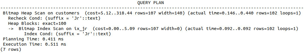
Figure 8.82: Query plan of the scan after creating an index on the suffix column

Again, the planning time is significantly elevated, but this cost is more than outweighed by the improvement in the execution time, which is reduced from 14.238 ms to 0.511 ms.

Activity 12: Implementing Hash Indexes

Solution

1. Use the EXPLAIN and ANALYZE commands to determine the planning time and cost, as well as the execution time and cost, of selecting all rows where the email subject is Shocking Holiday Savings On Electric Scooters:

   EXPLAIN ANALYZE SELECT * FROM emails where email_subject='Shocking Holiday Savings On Electric Scooters';

   The following output will be displayed:

   

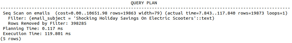
   Figure 8.83: Performance of sequential scan on the emails table

   The planning time is 0.117 ms and the execution time is 119.801ms. There is no cost in setting up the query, but there is a cost of 10,652 in executing it.

2. Use the EXPLAIN and ANALYZE commands to determine the planning time and cost, as well as the execution time and cost, of selecting all rows where the email subject is Black Friday. Green Cars.:

   EXPLAIN ANALYZE SELECT * FROM emails where email_subject='Black Friday. Green Cars.';

   The following output will be displayed:

   

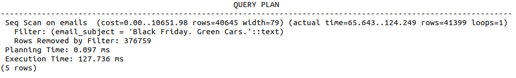
   Figure 8.84: Performance of a sequential scan looking for different email subject values

   Approximately 0.097 ms is spent on planning the query, with 127.736 ms being spent on executing it. This elevated execution time can be partially attributed to an increase in the number of rows being returned. Again, there is no setup cost, but a similar execution cost of 10,652.

3. Create a hash scan of the email subject field:

   CREATE INDEX ix_email_subject ON emails USING HASH(email_subject);

4. Repeat step 1 from the solution and compare both the outputs:

   EXPLAIN ANALYZE SELECT * FROM emails where email_subject='Shocking Holiday Savings On Electric Scooters';

   The following output will be displayed:

   

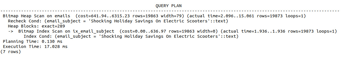
   Figure 8.85: Output of the query planner using a hash index

   The query plan shows that our newly created hash index is being used and has significantly reduced the execution time by over 100 ms, as well as the cost. There is a minor increase in the planning time and planning cost, all of which is easily outweighed by the reduction in execution time.

5. Repeat step 2 from the solution and compare both the outputs:

   EXPLAIN ANALYZE SELECT * FROM emails where email_subject='Black Friday. Green Cars.';

   The following is the output of the preceding code:

   

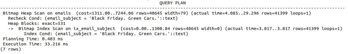
   Figure 8.86: Output of the query planner for a less-performant hash index

   Again, we can see a reduction in both planning and execution expenses. However, the reductions in the "Black Friday…" search are not as good as those achieved in the "Shocking Holiday Savings..." search. If we look in more detail, we can see that the scan on the index is approximately two times longer, but there are also about twice as many records in the latter example. From this, we can conclude that the increase is simply due to the increase in the number of records being returned by the query.

6. Create a hash scan of the customer_id field:

   CREATE INDEX ix_customer_id ON emails USING HASH(customer_id);

7. Use EXPLAIN and ANALYZE to estimate the time required to select all rows with a customer_id value greater than 100. What type of scan was used and why?

   EXPLAIN ANALYZE SELECT * FROM emails WHERE customer_id > 100;

   The following output will be displayed:

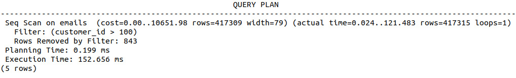
Figure 8.87: Query planner ignoring the hash index due to limitations

So, the final execution time comes to 152.656ms and the planning time comes to 0.199ms.

Activity 13: Implementing Joins

Solution

1. Open PostgreSQL and connect to the sqlda database:

   $ psql sqlda

2. Determine a list of customers (customer_id, first_name, and last_name) who had been sent an email, including information for the subject of the email and whether they opened and clicked on the email. The resulting table should include the customer_id, first_name, last_name, email_subject, opened, and clicked columns.

   sqlda=# SELECT customers.customer_id, customers.first_name, customers.last_name, emails.opened, emails.clicked FROM customers INNER JOIN emails ON customers.customer_id=emails.customer_id;

   The following screenshot shows the output of the preceding code:

   

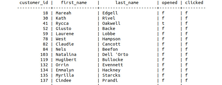
   Figure 8.88: Customers and emails join

3. Save the resulting table to a new table, customer_emails:

   sqlda=# SELECT customers.customer_id, customers.first_name, customers.last_name, emails.opened, emails.clicked INTO customer_emails FROM customers INNER JOIN emails ON customers.customer_id=emails.customer_id;

4. Find those customers who opened or clicked on an email:

   SELECT * FROM customer_emails WHERE clicked='t' and opened='t';

   The following figure shows the output of the preceding code:

   

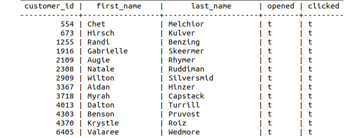
   Figure 8.89: Customers who had clicked on and opened emails

5. Find the customers who have a dealership in their city; customers who do not have a dealership in their city should have a blank value for the city column:

   sqlda=# SELECT customers.customer_id, customers.first_name, customers.last_name, customers.city FROM customers LEFT JOIN dealerships on customers.city=dealerships.city;

   This will display the following output:

   

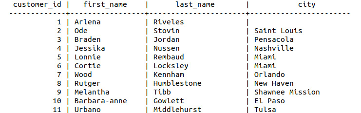
   Figure 8.90: Left join of customers and dealerships

6. Save these results to a table called customer_dealers:

   sqlda=# SELECT customers.customer_id, customers.first_name, customers.last_name, customers.city INTO customer_dealers FROM customers LEFT JOIN dealerships on customers.city=dealerships.city;

7. List those customers who do not have dealers in their city (hint: a blank field is NULL):

   sqlda=# SELECT * from customer_dealers WHERE city is NULL;

   The following figure shows the output of the preceding code:

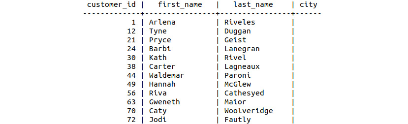
Figure 8.91: Customers without city information

The output shows the final list of customers in the cities where we have no dealerships.

Activity 14: Defining a Maximum Sale Function

Solution:

1. Connect to the sqlda database:

   $ psql sqlda

2. Create a function called max_sale that does not take any input arguments but returns a numeric value called big_sale:

   sqlda=# CREATE FUNCTION max_sale() RETURNS integer AS $big_sale$

3. Declare the big_sale variable and begin the function:

   sqlda$# DECLARE big_sale numeric;

   sqlda$# BEGIN

4. Insert the maximum sale amount into the big_sale variable:

   sqlda$# SELECT MAX(sales_amount) INTO big_sale FROM sales;

5. Return the value for big_sale:

   sqlda$# RETURN big_sale;

6. Close out the function with the LANGUAGE statement:

   sqlda$# END; $big_sale$

   sqlda-# LANGUAGE PLPGSQL;

7. Call the function to find what the biggest sale amount in the database is:

   sqlda=# SELECT MAX(sales_amount) FROM sales;

   The following figure shows the output of the preceding code:

Figure 8.92: Output of the maximum sales function call

The output is created from a function that determines the highest sale amount, that is, 115000, in the database.

Activity 15: Creating Functions with Arguments

Solution

1. Create the function definition for a function called avg_sales_window that returns a numeric value and takes a DATE value to specify the date in the form YYYY-MM-DD:

   sqlda=# CREATE FUNCTION avg_sales_window(from_date DATE, to_date DATE) RETURNS numeric AS $sales_avg$

2. Declare the return variable as a numeric data type and begin the function:

   sqlda$# DECLARE sales_avg numeric;

   sqlda$# BEGIN

3. Select the average sales amount into the return variable where the sales transaction date is greater than the specified date:

   sqlda$# SELECT AVG(sales_amount) FROM sales INTO sales_avg WHERE sales_transaction_date > from_date AND sales_transaction_date < to_date;

4. Return the function variable, end the function, and specify the LANGUAGE statement:

   sqlda$# RETURN sales_avg;

   sqlda$# END; $channel_avg$

   sqlda-# LANGUAGE PLPGSQL;

5. Use the function to determine the average sales value since 2013-04-12:

   sqlda=# SELECT avg_sales_window('2013-04-12', '2014-04-12');

   The following figure shows the output of the preceding code:

Figure 8.93: Output of average sales since the function call

The final output shows the average sales within specific dates, which comes to around 477.687.

Activity 16: Creating a Trigger to Track Average Purchases

Solution

1. Connect to the smalljoins database:

   $ psql smalljoins

2. Create a new table called avg_qty_log that is composed of an order_id integer field and an avg_qty numeric field:

   smalljoins=# CREATE TABLE avg_qty_log (order_id integer, avg_qty numeric);

3. Create a function called avg_qty that does not take any arguments but returns a trigger. The function computes the average value for all order quantities (order_info.qty) and inserts the average value along with the most recent order_id into avg_qty:

   smalljoins=# CREATE FUNCTION avg_qty() RETURNS TRIGGER AS $_avg$

   smalljoins$# DECLARE _avg numeric;

   smalljoins$# BEGIN

   smalljoins$# SELECT AVG(qty) INTO _avg FROM order_info;

   smalljoins$# INSERT INTO avg_qty_log (order_id, avg_qty) VALUES (NEW.order_id, _avg);

   smalljoins$# RETURN NEW;

   smalljoins$# END; $_avg$

   smalljoins-# LANGUAGE PLPGSQL;

4. Create a trigger called avg_trigger that calls the avg_qty function AFTER each row is inserted into the order_info table:

   smalljoins=# CREATE TRIGGER avg_trigger

   smalljoins-# AFTER INSERT ON order_info

   smalljoins-# FOR EACH ROW

   smalljoins-# EXECUTE PROCEDURE avg_qty();

5. Insert some new rows into the order_info table with quantities of 6, 7, and 8:

   smalljoins=# SELECT insert_order(3, 'GROG1', 6);

   smalljoins=# SELECT insert_order(4, 'GROG1', 7);

   smalljoins=# SELECT insert_order(1, 'GROG1', 8);

6. Look at the entries in avg_qty_log to see whether the average quantity of each order is increasing:

   smalljoins=# SELECT * FROM avg_qty_log;

   The following figure shows the output of the preceding code:

Figure 8.94: Average order quantity over time

With these orders and the entries in the log, we can see an increase in the average quantity of items per order.

Activity 17: Terminating a Long Query

Solution

1. Launch two separate SQL interpreters:

   C:> psql sqlda

2. In the first terminal, execute the sleep command with a parameter of 1000 seconds:

   sqlda=# SELECT pg_sleep(1000);

3. In the second terminal, identify the process ID of the sleep query:
   

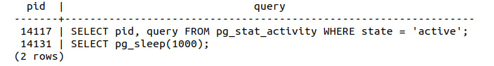
   Figure 8.95: Finding the pid value of pg_sleep

4. Using the pid value, force the sleep command to terminate using the pg_terminate_background command:

   Sqlda=# SELECT pg_terminate_backend(14131);

   The following figure shows the output of the preceding code:

   

   Figure 8.96: Forcefully terminating pg_sleep

5. Verify in the first terminal that the sleep command has been terminated. Notice the message returned by the interpreter:

   Sqlda=# SELECT pg_sleep(1000);

   This will display the following output:

Figure 8.97: Terminated pg_sleep process

We can see that the query is now terminated from the screenshot after using the pg_sleep command.

Chapter 9: Using SQL to Uncover the Truth – a Case Study

Activity 18: Quantifying the Sales Drop

Solution

1. Load the sqlda database:

   $ psql sqlda

2. Compute the daily cumulative sum of sales using the OVER and ORDER BY statements. Insert the results into a new table called bat_sales_growth:

   sqlda=# SELECT *, sum(count) OVER (ORDER BY sales_transaction_date) INTO bat_sales_growth FROM bat_sales_daily;

   The following table shows the daily cumulative sum of sales:

   

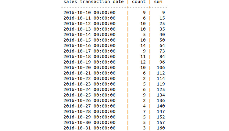
   Figure 9.48: Daily sales count

3. Compute a 7-day lag function of the sum column and insert all the columns of bat_sales_daily and the new lag column into a new table, bat_sales_daily_delay. This lag column indicates what the sales were like 1 week before the given record:

   sqlda=# SELECT *, lag(sum, 7) OVER (ORDER BY sales_transaction_date) INTO bat_sales_daily_delay FROM bat_sales_growth;

4. Inspect the first 15 rows of bat_sales_growth:

   sqlda=# SELECT * FROM bat_sales_daily_delay LIMIT 15;

   The following is the output of the preceding code:

   

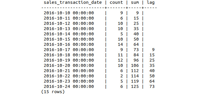
   Figure 9.49: Daily sales delay with lag

5. Compute the sales growth as a percentage, comparing the current sales volume to that of 1 week prior. Insert the resulting table into a new table called bat_sales_delay_vol:

   sqlda=# SELECT *, (sum-lag)/lag AS volume INTO bat_sales_delay_vol FROM bat_sales_daily_delay ;

   Note

   The percentage sales volume can be calculated via the following equation:

   (new_volume – old_volume) / old_volume

6. Compare the first 22 values of the bat_sales_delay_vol table:

   sqlda=# SELECT * FROM bat_sales_daily_delay_vol LIMIT 22;

   The delay volume for the first 22 entries can be seen in the following:

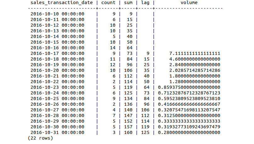
Figure 9.50: Relative sales volume of the scooter over 3 weeks

Looking at the output table, we can see four sets of information: the daily sales count, the cumulative sum of the daily sales count, the cumulative sum offset by 1 week (the lag), and the relative daily sales volume.

Activity 19: Analyzing the Difference in the Sales Price Hypothesis

Solution

1. Load the sqlda database:

   $ psql sqlda

2. Select the sales_transaction_date column from the 2013 Lemon sales and insert the column into a table called lemon_sales:

   sqlda=# SELECT sales_transaction_date INTO lemon_sales FROM sales WHERE product_id=3;

3. Count the sales records available for the 2013 Lemon by running the following query:

   sqlda=# SELECT count(sales_transaction_date) FROM lemon_sales;

   We can see that 16558 records are available:

   

   Figure 9.51: Sales records for the 2013 Lemon Scooter

4. Use the max function to check the latest sales_transaction_date column:

   sqlda=# SELECT max(sales_transaction_date) FROM lemon_sales;

   The following figure displays the sales_transaction_date column:

   

   Figure 9.52: Production between May 2013 and December 2018

5. Convert the sales_transaction_date column to a date type using the following query:

   sqlda=# ALTER TABLE lemon_sales ALTER COLUMN sales_transaction_date TYPE DATE;

   We are converting the datatype from DATE_TIME to DATE so as to remove the time information from the field. We are only interested in accumulating numbers, but just the date and not the time. Hence, it is easier just to remove the time information from the field.

6. Count the number of sales per day within the lemon_sales table and insert this figure into a table called lemon_sales_count:

   sqlda=# SELECT *, COUNT(sales_transaction_date) INTO lemon_sales_count FROM lemon_sales GROUP BY sales_transaction_date,lemon_sales.customer_id ORDER BY sales_transaction_date;

7. Calculate the cumulative sum of sales and insert the corresponding table into a new table labeled lemon_sales_sum:

   sqlda=# SELECT *, sum(count) OVER (ORDER BY sales_transaction_date) INTO lemon_sales_sum FROM lemon_sales_count;

8. Compute the 7-day lag function on the sum column and save the result to lemon_sales_delay:

   sqlda=# SELECT *, lag(sum, 7) OVER (ORDER BY sales_transaction_date) INTO lemon_sales_delay FROM lemon_sales_sum;

9. Calculate the growth rate using the data from lemon_sales_delay and store the resulting table in lemon_sales_growth. Label the growth rate column as volume:

   sqlda=# SELECT *, (sum-lag)/lag AS volume INTO lemon_sales_growth FROM lemon_sales_delay;

10. Inspect the first 22 records of the lemon_sales_growth table by examining the volume data:

    sqlda=# SELECT * FROM lemon_sales_growth LIMIT 22;

    The following table shows the sales growth:

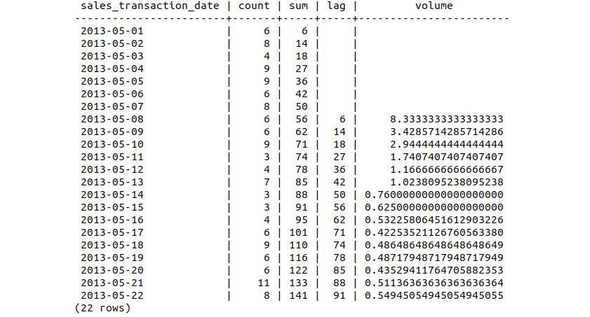
Figure 9.53: Sales growth of the Lemon Scooter

Similar to the previous exercise, we have calculated the cumulative sum, lag, and relative sales growth of the Lemon Scooter. We can see that the initial sales volume is much larger than the other scooters, at over 800%, and again finishes higher at 55%