Chapter 4

Aggregate Functions for Data Analysis

Learning Objectives

By the end of this chapter, you will be able to:

• Explain the conceptual logic of aggregation
• Identify the common SQL aggregate functions
• Use the GROUP BY clause to aggregate and combine groups of data for analysis
• Use the HAVING clause to filter aggregates
• Use aggregate functions to clean data and examine data quality

In this chapter, we will cover SQL's aggregate functions, which are powerful functions for summarizing data.

Introduction

In the previous chapter, we discussed how to use SQL to prepare datasets for analysis. Once the data is prepared, the next step is to analyze the data. Generally, data scientists and analytics professionals will try to understand the data by summarizing it and trying to find high-level patterns in the data. SQL can help with this task primarily through the use of aggregate functions: functions that take rows as input and return one number for each row. In this chapter, we will discuss how to use basic aggregate functions and how to derive statistics and other useful information from data using aggregate functions with GROUP BY. We will then use the HAVING clause to filter aggregates and see how to clean data and examine data quality using aggregate functions. Finally, we look at how to use aggregates to understand data quality

Aggregate Functions

With data, we are often interested in understanding the properties of an entire column or table as opposed to just seeing individual rows of data. As a simple example, let's say you were wondering how many customers ZoomZoom has. You could select all the data from the table and then see how many rows were pulled back, but it would be incredibly tedious to do so. Luckily, there are functions provided by SQL that can be used to do calculations on large groups of rows. These functions are called aggregate functions. The aggregate function takes in one or more columns with multiple rows and returns a number based on those columns. As an illustration, we can use the COUNT function to count how many rows there are in the customers table to figure out how many customers ZoomZoom has:

SELECT COUNT(customer_id) FROM customers;

The COUNT function will return the number of rows without a NULL value in the column. As the customer_id column is a primary key and cannot be NULL, the COUNT function will return the number of rows in the table. In this case, the query will return:

Figure 4.1: Customer count table

As shown here, the COUNT function works with a single column and counts how many non-NULL values it has. However, if every single column has at least one NULL value, then it would be impossible to determine how many rows there are. To get a count of the number of rows in that situation, you could alternatively use the COUNT function with an asterisk, (*), to get the total count of rows:

SELECT COUNT(*) FROM customers;

This query will also return 50,000.

Let's say, however, that what you were interested in was the number of unique states in the customer list. This answer could be queried using COUNT (DISTINCT expression):

SELECT COUNT(DISTINCT state) FROM customers;

This query creates the following output:

Figure 4.2: Count of distinct states

The following figure is a summary of the major aggregate functions used in SQL:

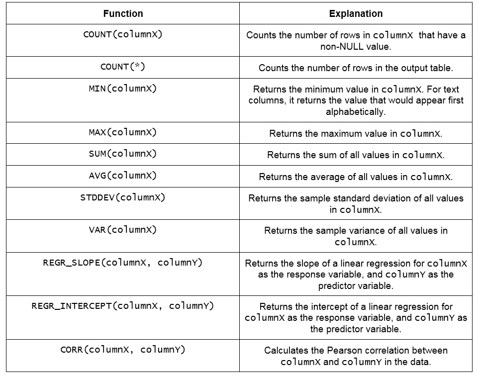
Figure 4.3: Major aggregate functions

Aggregate functions can also be used with the WHERE clause in order to calculate aggregate values for specific subsets of data. For example, if you wanted to know how many customers ZoomZoom had in California, you could use the following query:

SELECT COUNT(*) FROM customers WHERE state='CA';

This gives the following result:

Figure 4.4: The COUNT function used with the WHERE clause

You can also do arithmetic with aggregate functions. In the following query, you can divide the count of rows in the customers table by two like so:

SELECT COUNT(*)/2 FROM customers;

This query will return 25,000.

You can also use the aggregate functions with each other in mathematical ways. In the following query, instead of using the AVG function to calculate the average MSRP of products at ZoomZoom, you could "build" the AVG function using SUM and COUNT as follows:

SELECT SUM(base_msrp)::FLOAT/COUNT(*) AS avg_base_msrp FROM products

You should get the following result:

Figure 4.5: Average of the base MSRP

Note

The reason we have to cast the sum is that PostgreSQL treats integer division differently than float division. For example, dividing 7 by 2 as integers in PostgreSQL will give you 3. In order to get a more precise answer of 3.5, you have to cast one of the numbers to float.

Exercise 13: Using Aggregate Functions to Analyze Data

Here, we will analyze and calculate the price of a product using different aggregate functions. As you're always curious about the data at your company, you are interested in understanding some of the basic statistics around ZoomZoom product prices. You now want to calculate the lowest price, the highest price, the average price, and the standard deviation of the price for all the products the company has ever sold.

Note

For all exercises in this book, we will be using pgAdmin 4. All the exercises and activity are also available on GitHub: https://github.com/TrainingByPackt/SQL-for-Data-Analytics/tree/master/Lesson04.

To solve this problem, do the following:

1. Open your favorite SQL client and connect to the sqlda database.
2. Calculate the lowest, highest, average, and standard deviation of the price using the MIN, MAX, AVG, and STDDEV aggregate functions, respectively, from the products table:

   SELECT MIN(base_msrp), MAX(base_msrp), AVG(base_msrp), STDDEV(base_msrp)

   FROM products;

   The following is the output of the preceding code:

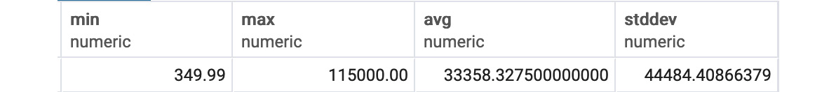
Figure 4.6: Statistics of the product price

We can see from the output that the minimum price is 349.99, the maximum price is 115000.00, the average price is 33358.32750, and the standard deviation of the price is 44484.408.

We have now used aggregate functions to understand the basic statistics of prices.

Aggregate Functions with GROUP BY

We have now used aggregate functions to calculate statistics for an entire column. However, often, we are not interested in the aggregate values for a whole table, but for smaller groups in the table. To illustrate, let's go back to the customers table. We know the total number of customers is 50,000. But we might want to know how many customers we have in each state. How would we calculate this?

We could determine how many states there are with the following query:

SELECT DISTINCT state FROM customers;

Once you have the list of states, you could then run the following query for each state:

SELECT COUNT(*) FROM customer WHERE state='{state}'

Although you can do this, it is incredibly tedious and can take an incredibly long time if there are many states. Is there a better way? There is, and it is through the use of the GROUP BY clause.

GROUP BY

GROUP BY is a clause that divides the rows of a dataset into multiple groups based on some sort of key specified in the GROUP BY clause. An aggregate function is then applied to all the rows within a single group to produce a single number. The GROUP BY key and the aggregate value for the group are then displayed in the SQL output. The following diagram illustrates this general process:

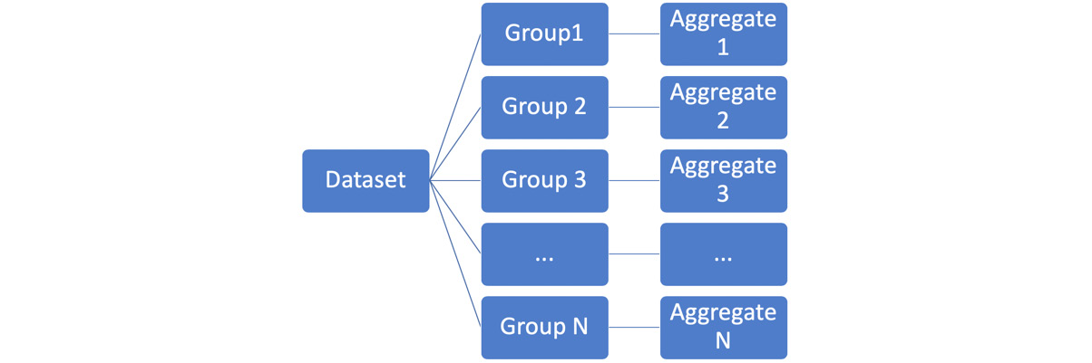
Figure 4.7: General GROUP BY computational model

In Figure 4.7, we can see that the dataset has multiple groups (Group 1, Group 2, …., Group N). Here, the Aggregate 1 function is applied to all the rows in Group1, the Aggregate 2 function is applied to all the rows in Group 2, and so on.

GROUP BY statements usually have the following structure:

SELECT {KEY}, {AGGFUNC(column1)} FROM {table1} GROUP BY {KEY}

Here, {KEY} is a column or a function on a column used to create individual groups, {AGGFUNC(column1)} is an aggregate function on a column that is calculated for all the rows within each group, and {table} is the table or set of joined tables from which rows are separated into groups.

To better illustrate this point, let's count the number of customers in each US state using a GROUP BY query. Using GROUP BY, a SQL user could count the number of customers in each state by querying:

SELECT state, COUNT(*) FROM customers GROUP BY state

The computational model looks like the following:

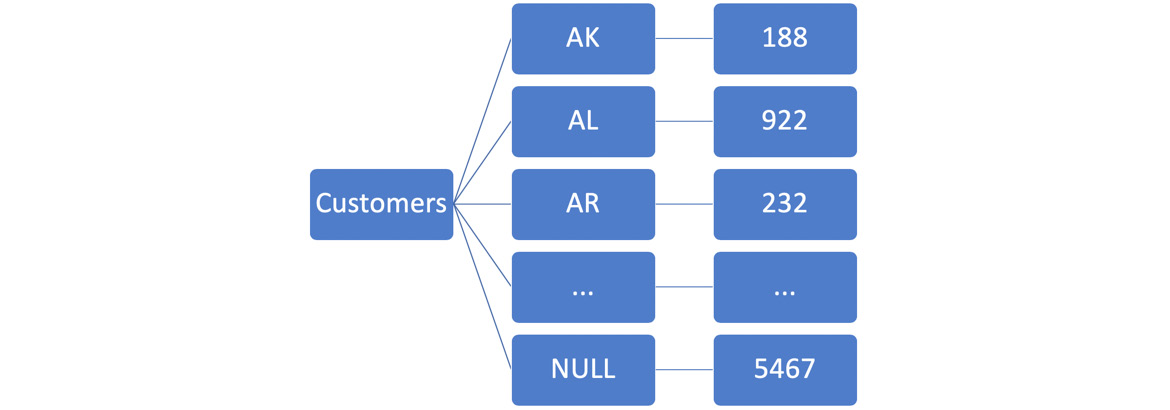
Figure 4.8: Customer count by the state computational model

Here, AK, AL, AR, and the other keys are abbreviations for US states.

You should get output similar to the following:

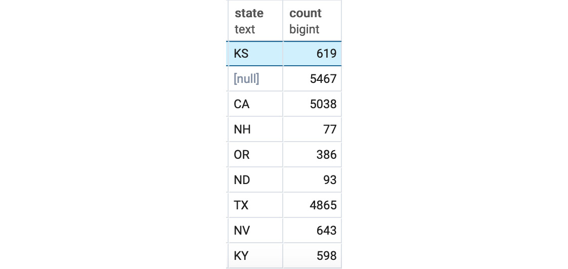
Figure 4.9: Customer count by the state query output

You can also use the column number to perform a GROUP BY operation:

SELECT state, COUNT(*) FROM customers

GROUP BY 1

If you want to return the output in alphabetical order, simply use the following query:

SELECT state, COUNT(*) FROM customers GROUP BY state ORDER BY state

Alternatively, we can write:

SELECT state, COUNT(*) FROM customers GROUP BY 1ORDER BY 1

Either of these queries will give you the following result:

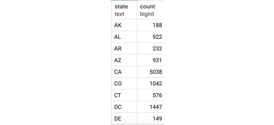
Figure 4.10: Customer count by the state query output in alphabetical order

Often, though, you may be interested in ordering the aggregates themselves. The aggregates can be ordered using ORDER BY as follows:

SELECT state, COUNT(*) FROM customers GROUP BY state ORDER BY COUNT(*)

This query gives the following output:

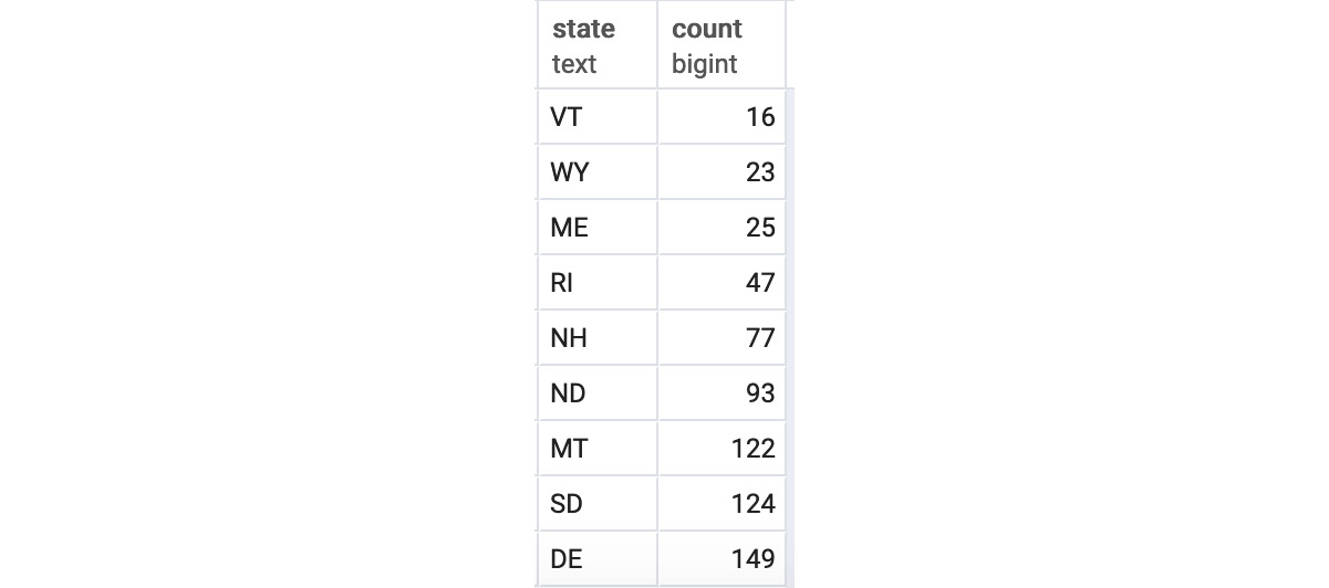
Figure 4.11: Customer count by the state query output in increasing order

You may also want to count only a subset of the data, such as the total number of male customers. To calculate the total number of male customers, you can use the following query:

SELECT state, COUNT(*) FROM customers WHERE gender='M' GROUP BY state ORDER BY state

This gives you the following output:

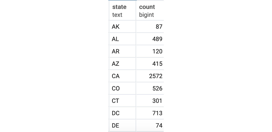
Figure 4.12: Male customer count by the state query output in alphabetical order

Multiple Column GROUP BY

While GROUP BY with one column is powerful, you can go even further and GROUP BY multiple columns. Let's say you wanted to get a count of not just the number of customers ZoomZoom had in each state, but also of how many male and female customers it had in each state. Multiple GROUP BY columns can query the answer as follows:

SELECT state, gender, COUNT(*) FROM customers GROUP BY state, genderORDER BY state, gender

This gives the following result:

Figure 4.13: Customer count by the state and gender query outputs in alphabetical order

Any number of columns can be used in a GROUP BY operation in this fashion.

Exercise 14: Calculating the Cost by Product Type Using GROUP BY

In this exercise, we will analyze and calculate the cost of products using aggregate functions and the GROUP BY clause. The marketing manager wants to know the minimum, maximum, average, and standard deviation of the price for each product type that ZoomZoom sells, for a marketing campaign. Follow these steps:

1. Open your favorite SQL client and connect to the sample database, sqlda.
2. Calculate the lowest, highest, average, and standard deviation price using the MIN, MAX, AVG, and STDDEV aggregate functions, respectively, from the products table and use GROUP BY to check the price of all the different product types:

   SELECT product_type, MIN(base_msrp), MAX(base_msrp), AVG(base_msrp), STDDEV(base_msrp)

   FROM products

   GROUP BY 1

   ORDER BY 1;

   You should get the following result:

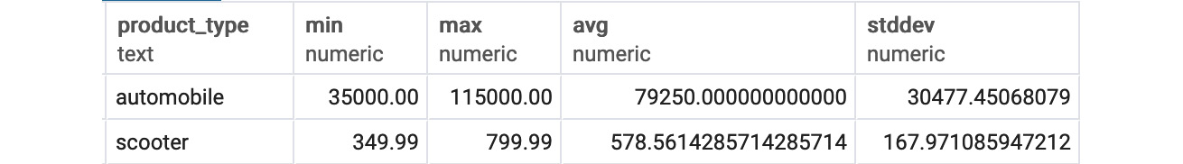
Figure 4.14: Basic price statistics by product type

From the preceding output, the marketing manager can check and compare the price of various products that ZoomZoom sells for the campaign.

In this exercise, we calculated the basic statistics by product type using aggregate functions and the GROUP BY clause.

Grouping Sets

Now, let's say you wanted to count the total number of customers you have in each state, while simultaneously, in the same aggregate functions, counting the total number of male and female customers you have in each state. How could you accomplish that? One way is by using the UNION ALL keyword we discussed in Chapter 2, The Basics of SQL for Analytics, like so:

(

SELECT state, NULL as gender, COUNT(*)

FROM customers

GROUP BY 1, 2

ORDER BY 1, 2

)

UNION ALL

(

(

SELECT state, gender, COUNT(*)

FROM customers

GROUP BY 1, 2

ORDER BY 1, 2

)

)

ORDER BY 1, 2

The query produces the following result:

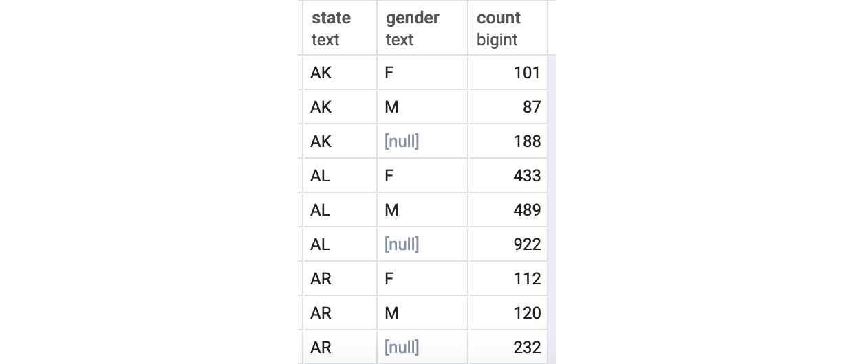
Figure 4.15: Customer count by the state and gender query outputs in alphabetical order

However, using UNION ALL is tedious and can be very difficult to write. An alternative way is to use grouping sets. Grouping sets allow a user to create multiple categories of viewing, similar to the UNION ALL statement we just saw. For example, using the GROUPING SETS keyword, you could rewrite the previous UNION ALL query as:

SELECT state, gender, COUNT(*)

FROM customers

GROUP BY GROUPING SETS (

(state),

(gender),

(state, gender)

)

ORDER BY 1, 2

This creates the same output as the previous UNION ALL query.

Ordered Set Aggregates

Up to this point, all the aggregates we have discussed did not depend on the order of the data. Using ORDER BY, we can order the data, but it was not required. However, there are a subset of aggregates statistics that do depend on the order of the column to calculate. For instance, the median of a column is something that requires the order of the data to be specified. For calculating these use cases, SQL offers a series of functions called ordered set aggregates functions. The following figure lists the major ordered-set aggregate functions:

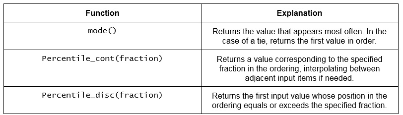
Figure 4.16: Major ordered set aggregate functions

The functions are used with the following format:

SELECT {ordered_set_function} WITHIN GROUP (ORDER BY {order_column})FROM {table};

Where {ordered_set_function} is the ordered set aggregate function, {order_column} is the column to order results for the function by, and {table} is the table the column is in.

To illustrate, let's say you wanted to calculate the median price of the products table. You could use the following query:

SELECT PERCENTILE_CONT(0.5) WITHIN GROUP (ORDER BY base_msrp) AS median

from products;

The reason we use 0.5 is because the median is the 50th percentile, which is 0.5 as a fraction. This gives the following result:

Figure 4.17: Median of Product Prices

With ordered set aggregate functions, we now have tools for calculating virtually any aggregate statistic of interest for a data set. In the next section, we look at how to use aggregates to deal with data quality.

The HAVING Clause

We can now perform all sorts of aggregate operations using GROUP BY. Sometimes, though, certain rows in aggregate functions may not be useful, and you may like to remove them from the query output. For example, when doing the customer counts, perhaps you are only interested in places that have at least 1,000 customers. Your first instinct may be to write something such as this:

SELECT state, COUNT(*)

FROM customers

WHERE COUNT(*)>=1,000

GROUP BY state

ORDER BY state

However, you will find that the query does not work and gives you the following error:

Figure 4.18: Error showing the query not working

In order to use filter on aggregate functions, you need to use a new clause, HAVING. The HAVING clause is similar to the WHERE clause, except it is specifically designed for GROUP BY queries. The general structure of a GROUP BY operation with a HAVING statement is:

SELECT {KEY}, {AGGFUNC(column1)}

FROM {table1}

GROUP BY {KEY}

HAVING {OTHER_AGGFUNC(column2)_CONDITION}

Here, {KEY} is a column or function on a column that is used to create individual groups, {AGGFUNC(column1)} is an aggregate function on a column that is calculated for all the rows within each group, {table} is the table or set of joined tables from which rows are separated into groups, and {OTHER_AGGFUNC(column2)_CONDITION} is a condition similar to what you would put in a WHERE clause involving an aggregate function.

Exercise 15: Calculating and Displaying Data Using the HAVING Clause

In this exercise, we will calculate and display data using the HAVING clause. The sales manager of ZoomZoom wants to know the customer count for the states that have at least 1,000 customers who have purchased any product from ZoomZoom. Help the manager to extract the data.

To solve this problem, do the following:

1. Open your favorite SQL client and connect to the sqlda database.
2. Calculate the customer count by the state with at least 1000 customers using the HAVING clause:

   SELECT state, COUNT(*)

   FROM customers

   GROUP BY state

   HAVING COUNT(*)>=1,000

   ORDER BY state

   This query will then give you the following output:

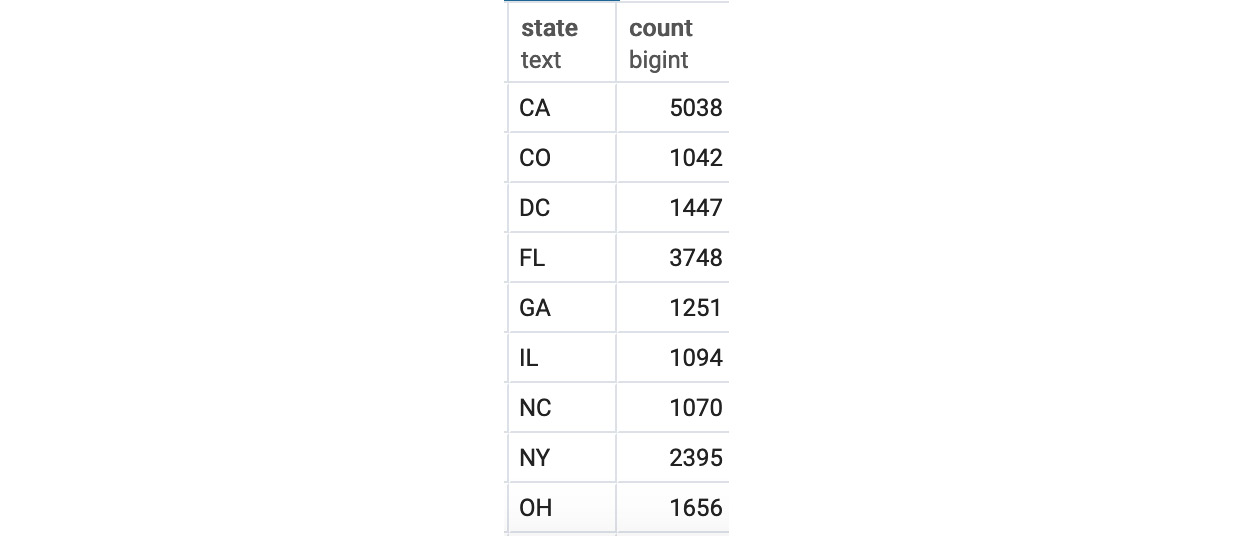
Figure 4.19: Customer count by the state with at least 1,000 customers

We can see the states that have more than 1,000 ZoomZoom customers, with CA having 5038, the highest number of customers, and CO having 1042, the lowest number of customers.

In this exercise, we used the HAVING clause to calculate and display data more efficiently.

Using Aggregates to Clean Data and Examine Data Quality

In Chapter 2, The Basics of SQL for Analytics, we discussed how SQL can be used to clean data. While the techniques in Chapter 2, The Basics of SQL for Analytics for Analytics, do an excellent job of cleaning data, aggregates add a number of techniques that can make cleaning data even easier and more comprehensive. In this section, we will look at some of these techniques.

Finding Missing Values with GROUP BY

As mentioned in Chapter 2, The Basics of SQL for Analytics, one of the biggest issues with cleaning data is dealing with missing values. While in Chapter 2, The Basics of SQL for Analytics, we discussed how to find missing values and how we could get rid of them, we did not say too much about how we could determine the extent of missing data in a dataset. Primarily, it was because we did not have the tools to deal with summarizing information in a dataset – that is, until this chapter.

Using aggregates, identifying the amount of missing data can tell you not only which columns have missing data, but also whether columns are even usable because so much of the data is missing. Depending on the extent of missing data, you will have to determine whether it makes the most sense to delete rows with missing data, fill in missing values, or to just delete columns as they do not have enough data to make definitive conclusions.

The easiest way to determine whether a column is missing values is to use a modified CASE WHEN statement with the SUM and COUNT functions to determine what percentage of data is missing. Generally speaking, the query looks as follows:

SELECT SUM(CASE WHEN {column1} IS NULL OR {column1} IN ({missing_values}) THEN 1 ELSE 0 END)::FLOAT/COUNT(*)

FROM {table1}

Here, {column1} is the column that you want to check for missing values, {missing_values} is a comma-separated list of values that are considered missing, and {table1} is the table or subquery with the missing values.

Based on the results of this query, you may have to vary your strategy for dealing with missing data. If a very small percentage of your data is missing (<1%), then you might consider just filtering out or deleting the missing data from your analysis. If some of your data is missing (<20%), you may consider filling in your missing data with a typical value, such as the mean or the mode, to perform an accurate analysis. If, however, more than 20% of your data is missing, you may have to remove the column from your data analysis, as there would not be enough accurate data to make accurate conclusions based on the values in the column.

Let's look at missing data in the customers table. Specifically, let's look at the missing data in the street_address column with the following query:

SELECT SUM(CASE WHEN state IS NULL OR state IN ('') THEN 1 ELSE 0 END)::FLOAT/COUNT(*)

AS missing_state

FROM customers;

This gives the following output:

Figure 4.20: Customer count by the state with at least 1,000 customers

As seen here, a little under 11% of the state data is missing. For analysis purposes, you may want to consider these customers are from CA, as CA is the most common state in the data. However, the far more accurate thing to do would be to find and fill in the missing data.

Measuring Data Quality with Aggregates

One of the major themes you will find in data analytics is that analysis is fundamentally only useful when there is a strong variation in data. A column where every value is exactly the same is not a particularly useful column. To this end, it often makes sense to determine how many distinct values there are in a column. To measure the number of distinct values in a column, we can use the COUNT DISTINCT function to find how many distinct values there are. The structure of such a query would look like this:

SELECT COUNT (DISTINCT {column1})

FROM {table1}

Here, {column1} is the column you want to count and {table1} is the table with the column.

Another common task that you might want to do is determine whether every value in a column is unique. While in many cases this can be solved by setting a column with a PRIMARY KEY constraint, this may not always be possible. To solve this problem, we can write the following query:

SELECT COUNT (DISTINCT {column1})=COUNT(*)

FROM {table1}

Here, {column1} is the column you want to count and {table1} is the table with the column. If this query returns True, then the column has a unique value for every single row; otherwise, at least one of the values is repeated. If values are repeated in a column that you are expecting to be unique, there may be some issues with data ETL (Extract, Transform, Load) or maybe there is a join that has caused a row to be repeated.

As a simple example, let's verify that the customer_id column in customers is unique:

SELECT COUNT (DISTINCT customer_id)=COUNT(*) AS equal_ids

FROM customers;

This query gives the following output:

Figure 4.21: Checking whether every row has a unique customer ID

Activity 6: Analyzing Sales Data Using Aggregate Functions

The goal of this activity is to analyze data using aggregate functions. The CEO, COO, and CFO of ZoomZoom would like to gain some insights on what might be driving sales. Now that the company feels they have a strong enough analytics team with your arrival. The task has been given to you, and your boss has politely let you know that this project is the most important project the analytics team has worked on:

1. Open your favorite SQL client and connect to the sqlda database.
2. Calculate the total number of unit sales the company has done.
3. Calculate the total sales amount in dollars for each state.
4. Identify the top five best dealerships in terms of the most units sold (ignore internet sales).
5. Calculate the average sales amount for each channel, as seen in the sales table, and look at the average sales amount first by channel sales, then by product_id, and then by both together.

Expected Output:

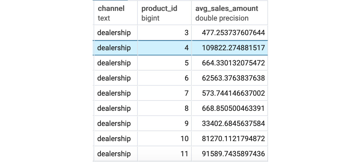
Figure 4.22: Sales after the GROUPING SETS channel and product_id

Note

The solution for the activity can be found on page 322.

Summary

In this chapter, we learned about the incredible power of aggregate functions. We learned about several of the most common aggregate functions and how to use them. We then used the GROUP BY clause and saw how it can be used to divide datasets into groups and calculate summary statistics for each group. We then learned how to use the HAVING clause to further filter a query. Finally, we used aggregate functions to help us clean data and analyze data quality.

In the next chapter, we will learn about a close cousin of aggregate functions, window functions, and see how they can be utilized to understand data.