Learning Objectives
By the end of this chapter, you will be able to:
- Assemble multiple tables and queries together into a dataset
- Transform and clean data using SQL functions
- Remove duplicate data using DISTINCT and DISTINCT ON
In this chapter, we will learn to clean and prepare our data for analysis using SQL techniques.
Introduction
In the previous chapter, we discussed the basics of SQL and how to work with individual tables in SQL. We also used CRUD (create, read, update and delete) operations on a table. These tables are the foundation for all the work undertaken in analytics. One of the first tasks implemented in analytics is to create clean datasets. According to Forbes, it is estimated that, almost 80% of the time spent by analytics professionals involves preparing data for use in analysis and building models with unclean data which harms analysis by leading to poor conclusions. SQL can help in this tedious but important task, by providing ways to build datasets which are clean, in an efficient manner. We will start by discussing how to assemble data using JOINs and UNIONs. Then, we will use different functions, such as CASE WHEN, COALESCE, NULLIF, and LEAST/GREATEST, to clean data. We will then discuss how to transform and remove duplicate data from queries using the DISTINCT command.
Assembling Data
Connecting Tables Using JOIN
In Chapter 2, The Basics of SQL for Analytics, we discussed how we can query data from a table. However, the majority of the time, the data you are interested in is spread across multiple tables. Fortunately, SQL has methods for bringing related tables together using the JOIN keyword.
To illustrate, let's look at two tables in our database – dealerships and salespeople. In the salespeople table, we observe that we have a column called dealership_id. This dealership_id column is a direct reference to the dealership_id column in the dealerships table. When table A has a column that references the primary key of table B, the column is said to be a foreign key to table A. In this case, the dealership_id column in salespeople is a foreign key to the dealerships table.
Note
Foreign keys can also be added as a column constraint to a table in order to improve the integrity of the data by making sure that the foreign key never contains a value that cannot be found in the referenced table. This data property is known as referential integrity. Adding foreign key constraints can also help to improve performance in some databases. Foreign key constraints are beyond the scope of this book and, in most instances, your company's data engineers and database administrators will deal with these details. You can learn more about foreign key constraints in the PostgreSQL documentation at the following link: https://www.postgresql.org/docs/9.4/tutorial-fk.html.
As these tables are related, you can perform some interesting analyses with these two tables. For instance, you may be interested in determining which salespeople work at a dealership in California. One way of retrieving this information is to first query which dealerships are located in California using the following query:
SELECT *
FROM dealerships
WHERE state='CA';
This query should give you the following results:

Figure 3.1: Dealerships in California
Now that you know that the only two dealerships in California have IDs of 2 and 5, respectively, you can then query the salespeople table as follows:
SELECT *
FROM salespeople
WHERE dealership_id in (2, 5)
ORDER BY 1;
The results will be similar to the following:
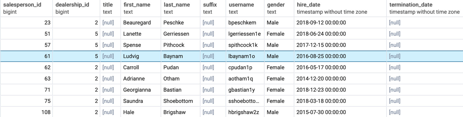
Figure 3.2: Salespeople in California
While this method gives you the results you want, it is tedious to perform two queries to get these results. What would make this query easier would be to somehow add the information from the dealerships table to the salespeople table and then filter for users in California. SQL provides such a tool with the JOIN clause. The JOIN clause is a SQL clause that allows a user to join one or more tables together based on distinct conditions.
Types of Joins
In this chapter, we will discuss three fundamental joins, which are illustrated in Figure 3.3: inner joins, outer joins, and cross joins:
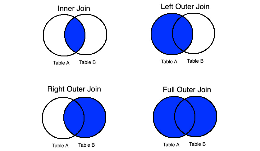
Figure 3.3: Major types of joins
INNER JOIN
The inner join connects rows in different tables together based on a condition known as the join predicate. In many cases, the join predicate is a logical condition of equality. Each row in the first table is compared against every other row in the second table. For row combinations that meet the inner join predicate, that row is returned in the query. Otherwise, the row combination is discarded.
Inner joins are usually written in the following form:
SELECT {columns}
FROM {table1}
INNER JOIN {table2} ON {table1}.{common_key_1}={table2}.{common_key_2}
Here, {columns} are the columns you want to get from the joined table, {table1} is the first table, {table2} is the second table, {common_key_1} is the column in {table1} you want to join on, and {common_key_2} is the column in {table2} to join on.
Now, let's go back to the two tables we discussed – dealerships and salespeople. As mentioned earlier, it would be good if we could append the information from the dealerships table to the salespeople table in order to know which state each dealer works in. For the time being, let's assume that all the salespeople IDs have a valid dealership_id.
Note
At this point in the book, you do not have the necessary skills to verify that every dealership ID is valid in the salespeople table, and so we assume it. However, in real-world scenarios, it will be important for you to validate these things on your own. Generally speaking, there are very few datasets and systems that guarantee clean data.
We can join the two tables using an equal's condition in the join predicate, as follows:
SELECT *
FROM salespeople
INNER JOIN dealerships
ON salespeople.dealership_id = dealerships.dealership_id
ORDER BY 1;
This query will produce the following output:
Figure 3.4: Salespeople table joined to the dealerships table
As you can see in the preceding output, the table is the result of joining the salespeople table to the dealerships table (note also that the first table listed in the query, salespeople, is on the left-hand side of the result, while the dealerships table is on the right-hand side. This is important to understand for the next section). More specifically, dealership_id in the salespeople table matches the dealership_id, in the dealerships table. This shows how the join predicate is met. By running this join query, we have effectively created a new "super dataset" consisting of the two tables merged together where the two dealership_id columns are equal.
We can now query this "super-dataset" the same way we would query one large table using the clauses and keywords from Chapter 1, Understanding and Describing Data. For example, going back to our multi-query issue to determine which sales query works in California, we can now address it with one easy query:
SELECT *
FROM salespeople
INNER JOIN dealerships
ON salespeople.dealership_id = dealerships.dealership_id
WHERE dealerships.state = 'CA'
ORDER BY 1
This gives us the following output:

Figure 3.5: Salespeople in California with one query
Careful readers will observe that the output in Figure 3.2 and Figure 3.5 are nearly identical, with the exception being that the table in Figure 3.5 has dealerships' data appended as well. If we want to isolate just the salespeople table portion of this, we can select the salespeople columns using the following star syntax:
SELECT salespeople.*
FROM salespeople
INNER JOIN dealerships
ON dealerships.dealership_id = salespeople.dealership_id
WHERE dealerships.state = 'CA'
ORDER BY 1;
There is one other shortcut that can help when writing statements with several join clauses: you can alias table names so that you do not have to type out the entire name of the table every time. Simply write the name of the alias after the first mention of the table after the join clause, and you can save a decent amount of typing. For instance, for the last preceding query, if we wanted to alias salespeople with s and dealerships with d, you could write the following statement:
SELECT s.*
FROM salespeople s
INNER JOIN dealerships d
ON d.dealership_id = s.dealership_id
WHERE d.state = 'CA'
ORDER BY 1;
Alternatively, you can also put the AS keyword between the table name and alias to make the alias more explicit:
SELECT s.*
FROM salespeople AS s
INNER JOIN dealerships AS d
ON d.dealership_id = s.dealership_id
WHERE d.state = 'CA'
ORDER BY 1;
Now that we have cleared up the basics of inner joins, we will discuss outer joins.
OUTER JOIN
As discussed, inner joins will only return rows from the two tables, and only if the join predicate is met for both rows. Otherwise, no rows from either table are returned. Sometimes, however, we want to return all rows from one of the tables regardless of whether the join predicate is met. In this case, the join predicate is not met; the row for the second table will be returned as NULL. These joins, where at least one table will be represented in every row after the join operation, are known as outer joins.
Outer joins can be classified into three categories: left outer joins, right outer joins, and full outer joins.
Left outer joins are where the left table (that is, the table mentioned first in a join clause) will have every row returned. If a row from the other table is not found, a row of NULL is returned. Left outer joins are performed by using the LEFT OUTER JOIN keywords followed by a join predicate. This can also be written in short as LEFT JOIN. To show how left outer joins work, let's examine two tables: the customers tables and the emails table. For the time being, assume that not every customer has been sent an email, and we want to mail all customers who have not received an email. We can use outer joins to make that happen. Let's do a left outer join between the customer table on the left and the emails table on the right. To help manage output, we will only limit it to the first 1,000 rows. The following code snippet is utilized:
SELECT *
FROM customers c
LEFT OUTER JOIN emails e ON e.customer_id=c.customer_id
ORDER BY c.customer_id
LIMIT 1000;
Following is the output of the preceding code:
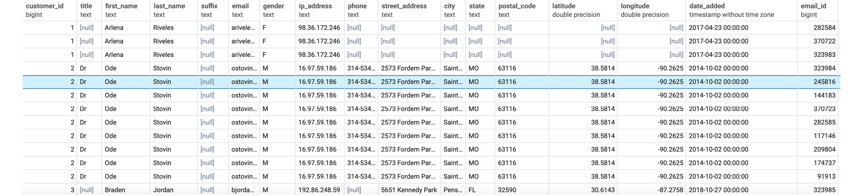
Figure 3.6: Customers left-joined to emails
When you look at the output of the query, you should see that entries from the customer table are present. However, for some of the rows, such as for customer row 27 which can be seen in Figure 3.7, the columns belonging to the emails table are completely full of nulls. This arrangement explains how the outer join is different from the inner join. If the inner join was used, the customer_id column would not be blank. This query, however, is still useful because we can now use it to find people who have never received an email. Because those customers who were never sent an email have a null customer_id column in the emails table, we can find all of these customers by checking the customer_id column in the emails table as follows:
SELECT *
FROM customers c
LEFT OUTER JOIN emails e ON c.customer_id = e.customer_id
WHERE e.customer_id IS NULL
ORDER BY c.customer_id
LIMIT 1000
We then get the following output:
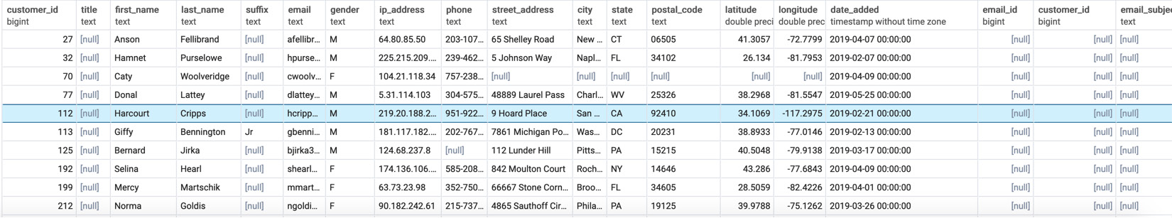
Figure 3.7: Customers with no emails sent
As you can see, all entries are blank in the customer_id column, indicating that they have not received any emails. We could simply grab the emails from this join to get all customers who have not received an email.
A right outer join is very similar to a left join, except the table on the "right" (the second listed table) will now have every row show up, and the "left" table will have NULLs if the join condition is not met. To illustrate, let's "flip" the last query by right-joining the emails table to the customers table with the following query:
SELECT *
FROM emails e
RIGHT OUTER JOIN customers c ON e.customer_id=c.customer_id
ORDER BY c.customer_id
LIMIT 1000;
When you run this query, you will get something similar to the following result:
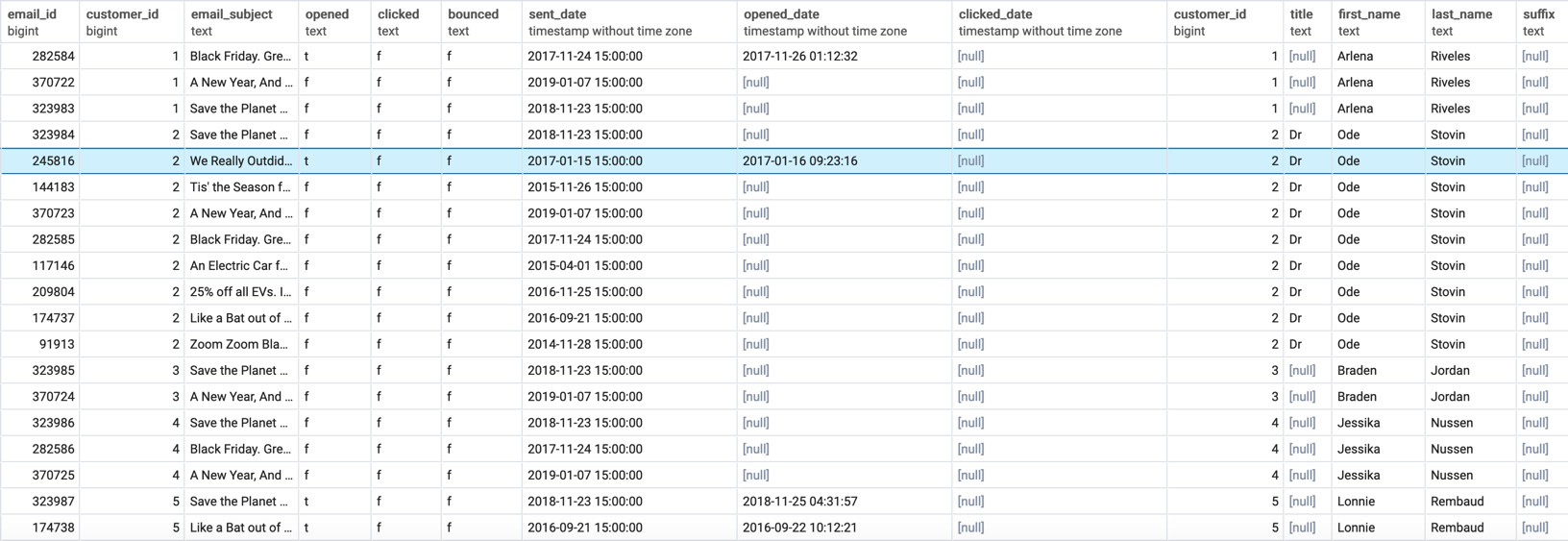
Figure 3.8: Emails right-joined to customers table
Notice that this output is similar to what was produced in Figure 3.7, except that the data from the emails table is now on the left-hand side, and the data from the customers table is on the right-hand side. Once again, customer_id 27 has NULL for the email. This shows the symmetry between a right join and a left join.
Finally, there is the full outer join. The full outer join will return all rows from the left and right tables, regardless of whether the join predicate is matched. For rows where the join predicate is met, the two rows are combined in a group. For rows where they are not met, the row has NULL filled in. The full outer join is invoked by using the FULL OUTER JOIN clause, followed by a join predicate. Here is the syntax of this join:
SELECT *
FROM email e
FULL OUTER JOIN customers c
ON e.customer_id=c.customer_id;
In this section, we learned how to implement three different outer joins. In the next section, we will work with the cross join.
CROSS JOIN
The final type of join we will discuss in this book is the cross join. The cross join is mathematically what is also referred to as the Cartesian product – it returns every possible combination of rows from the "left" table and the "right" table. It can be invoked using a CROSS JOIN clause, followed by the name of the other table. For instance, let's take the example of the products table.
Let's say we wanted to know every possible combination of two products you could create from a given set of products (like the one found in the products table) in order to create a two-month giveaway for marketing purposes. We can use a cross join to get the answer to the question using the following query:
SELECT p1.product_id, p1.model, p2.product_id, p2.model
FROM products p1 CROSS JOIN products p2;
The output of this query is as follows:
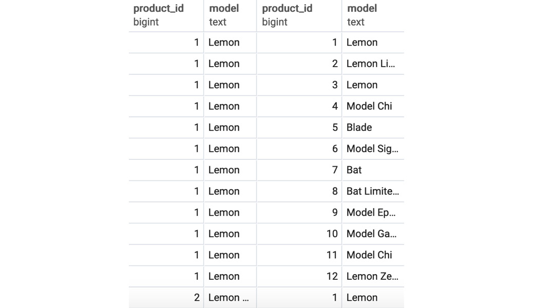
Figure 3.9: Cross join of a product to itself
You will observe that, in this particular case, we joined a table to itself. This is a perfectly valid operation and is also known as a self join. The result of the query has 144 rows, which is the equivalent of multiplying the 12 products by the same number (12 * 12). We can also see that there is no need for a join predicate; indeed, a cross join can simply be thought of as just an outer join with no conditions for joining.
In general, cross joins are not used in practice, and can also be very dangerous if you are not careful. Cross joining two large tables together can lead to the origination of hundreds of billions of rows, which can stall and crash a database. Take care when using them.
Note
To learn more about joins, check out the PostgreSQL documentation here: https://www.postgresql.org/docs/9.1/queries-table-expressions.html.
Up to this point, we have covered the basics of using joins to bring tables together. We will now talk about methods for joining queries together in a dataset.
Exercise 10: Using Joins to Analyze Sales Dealership
The head of sales at your company would like a list of all customers who bought a car. We need to create a query that will return all customer IDs, first names, last names, and valid phone numbers of customers who purchased a car.
Note
For all exercises in this book, we will be using pgAdmin 4. All the code files for the exercises and the activity in this chapter are also available on GitHub: https://github.com/TrainingByPackt/SQL-for-Data-Analytics/tree/master/Lesson03.
To solve this problem, do the following:
- Open your favorite SQL client and connect to the sqlda database.
- Use inner join to bring the tables' sales and customers together, which returns data for the following: customer IDs, first names, last names, and valid phone numbers:
SELECT c.customer_id,
c.first_name,
c.last_name,
c.phone
FROM sales s
INNER JOIN customers c ON c.customer_id=s.customer_id
INNER JOIN products p ON p.product_id=s.product_id
WHERE p.product_type='automobile'
AND c.phone IS NOT NULL
You should get an output similar to the following:
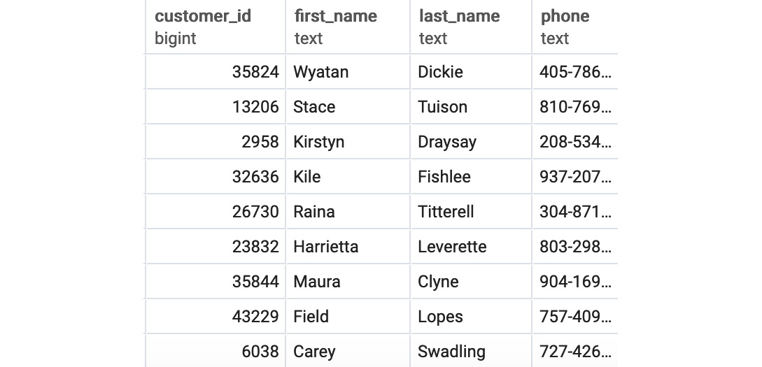
Figure 3.10: Customers who bought a car
We can see that after running the query, we were able to join the data from the tables sales and customers and obtain a list of customers who bought a car.
In this exercise, using joins, we were able to bring together related data easily and efficiently.
Subqueries
As of now, we have been pulling data from tables. However, you may have observed that all SELECT queries produce tables as an output. Knowing this, you may wonder whether there is some way to use the tables produced by SELECT queries instead of referencing an existing table in your database. The answer is yes. You can simply take a query, insert it between a pair of parentheses, and give it an alias. For example, if we wanted to find all the salespeople working in California, we could have written the query using the following alternative:
SELECT *
FROM salespeople
INNER JOIN (
SELECT * FROM dealerships
WHERE dealerships.state = 'CA'
) d
ON d.dealership_id = salespeople.dealership_id
ORDER BY 1
Here, instead of joining the two tables and filtering for rows with the state equal to 'CA', we first find the dealerships where the state equals 'CA' and then inner join the rows in that query to salespeople.
If a query only has one column, you can use a subquery with the IN keyword in a WHERE clause. For example, another way to extract the details from the salespeople table using the dealership ID for the state of California would be as follows:
SELECT *
FROM salespeople
WHERE dealership_id IN (
SELECT dealership_id FROM dealerships
WHERE dealerships.state = 'CA'
)
ORDER BY 1
As all these examples show, it's quite easy to write the same query using multiple techniques. In the next section, we will talk about unions.
Unions
So far, we have been talking about how to join data horizontally. That is, with joins, new columns are effectively added horizontally. However, we may be interested in putting multiple queries together vertically; that is, by keeping the same number of columns but adding multiple rows. An example may help to clarify this.
Let's say you wanted to visualize the addresses of dealerships and customers using Google Maps. To do this, you would need both the addresses of customers and dealerships You could build a query with all customer addresses as follows:
SELECT street_address, city, state, postal_code
FROM customers
WHERE street_address IS NOT NULL;
You could also retrieve dealership addresses with the following query:
SELECT street_address, city, state, postal_code
FROM dealerships
WHERE street_address IS NOT NULL;
However, it would be nice if we could assemble the two queries together into one list with one query. This is where the UNION keyword comes into play. Using the two previous queries, we could create the query:
(
SELECT street_address, city, state, postal_code
FROM customers
WHERE street_address IS NOT NULL
)
UNION
(
SELECT street_address, city, state, postal_code
FROM dealerships
WHERE street_address IS NOT NULL
)
ORDER BY 1;
This produces the following output:
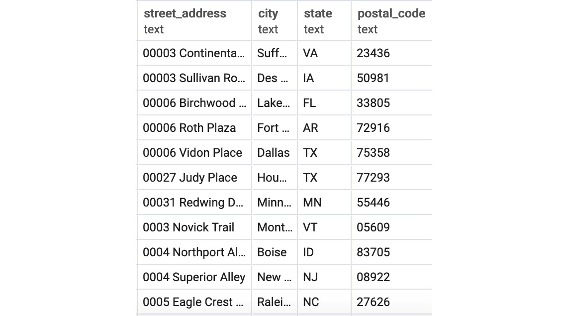
Figure 3.11: Union of Addresses
There are some caveats to using UNION. First, UNION requires that the subqueries therein have the same name columns and the same data types for the column. If it does not, the query will not run. Second, UNION technically may not return all the rows from its subqueries. UNION, by default, removes all duplicate rows in the output. If you want to retain the duplicate rows, it is preferable to use the UNION ALL keyword.
Exercise 11: Generating an Elite Customer Party Guest List using UNION
In this exercise, we will assemble two queries using unions. In order to help build up marketing awareness for the new Model Chi, the marketing team would like to throw a party for some of ZoomZoom's wealthiest customers in Los Angeles, CA. To help facilitate the party, they would like you to make a guest list with ZoomZoom customers who live in Los Angeles, CA, as well as salespeople who work at the ZoomZoom dealership in Los Angeles, CA. The guest list should include the first name, the last name, and whether the guest is a customer or an employee.
To solve this problem, execute the following:
- Open your favorite SQL client and connect to the sqlda database.
- Write a query that will make a list of ZoomZoom customers and company employees who live in Los Angeles, CA. The guest list should contain the first name, the last name, and whether the guest is a customer or an employee:
(
SELECT first_name, last_name, 'Customer' as guest_type
FROM customers
WHERE city='Los Angeles'
AND state='CA'
)
UNION
(
SELECT first_name, last_name, 'Employee' as guest_type
FROM salespeople s
INNER JOIN dealerships d ON d.dealership_id=s.dealership_id
WHERE d.city='Los Angeles'
AND d.state='CA'
)
You should get the following output:
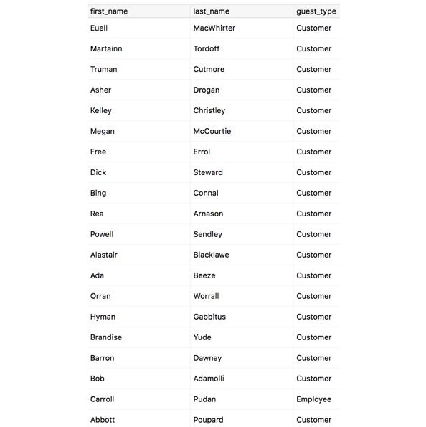
Figure 3.12: Customer and employee guest list in Los Angeles, CA
We can see the guest list of customers and employees from Los Angeles, CA after running the UNION query.
In the exercise, we used the UNION keyword to combine rows from different queries effortlessly.
Common Table Expressions
Common table expressions are, in a certain sense, just a different version of subqueries. Common table expressions establish temporary tables by using the WITH clause. To understand this clause better, let's have a look at the following query:
SELECT *
FROM salespeople
INNER JOIN (
SELECT * FROM dealerships
WHERE dealerships.state = 'CA'
) d
ON d.dealership_id = salespeople.dealership_id
ORDER BY 1
This could be written using common table expressions as follows:
WITH d as (
SELECT * FROM dealerships
WHERE dealerships.state = 'CA'
)
SELECT *
FROM salespeople
INNER JOIN d ON d.dealership_id = salespeople.dealership_id
ORDER BY 1;
The one advantage of common table expressions is that they are recursive. Recursive common table expressions can reference themselves. Because of this feature, we can use them to solve problems that other queries cannot. However, recursive common table expressions are beyond the scope of this book.
Now that we know several ways to join data together across a database, we will look at how to transform the data from these outputs.
Transforming Data
Often, the raw data presented in a query output may not be in the form we would like it to be. We may want to remove values, substitute values, or map values to other values. To accomplish these tasks, SQL provides a wide variety of statements and functions. Functions are keywords that take in inputs such as a column or a scalar value and change those inputs into some sort of output. We will discuss some very useful functions for cleaning data in the following sections.
CASE WHEN
CASE WHEN is a function that allows a query to map various values in a column to other values. The general format of a CASE WHEN statement is:
CASE WHEN condition1 THEN value1
WHEN condition2 THEN value2
…
WHEN conditionX THEN valueX
ELSE else_value END
Here, condition1 and condition2, through conditionX, are Boolean conditions; value1 and value2, through valueX, are values to map the Boolean conditions; and else_value is the value that is mapped if none of the Boolean conditions are met. For each row, the program starts at the top of the CASE WHEN statement and evaluates the first Boolean condition. The program then runs through each Boolean condition from the first one. For the first condition from the start of the statement that evaluates as true, the statement will return the value associated with that condition. If none of the statements evaluate as true, then the value associated with the ELSE statement will be returned.
As an example, let's say you wanted to return all rows for customers from the customers table. Additionally, you would like to add a column that labels a user as being an Elite Customer if they live in postal code 33111, or as a Premium Customer if they live in postal code 33124. Otherwise, it will mark the customer as a Standard Customer. This column will be called customer_type. We can create this table by using a CASE WHEN statement as follows:
SELECT *,
CASE WHEN postal_code='33111' THEN 'Elite Customer'
CASE WHEN postal_code='33124' THEN 'Premium Customer'
ELSE 'Standard Customer' END
AS customer_type
FROM customers;
This query will give the following output:
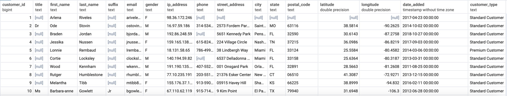
Figure 3.13: Customer type query
As you can see in the preceding table, there is a column called customer_type indicating the type of customer a user is. The CASE WHEN statement effectively mapped a postal code to a string describing the customer type. Using a CASE WHEN statement, you can map values in any way you please.
Exercise 12: Using the CASE WHEN Function to Get Regional Lists
The aim is to create a query that will map various values in a column to other values. The head of sales has an idea to try and create specialized regional sales teams that will be able to sell scooters to customers in specific regions, as opposed to generic sales teams. To make his idea a reality, he would like a list of all customers mapped to regions. For customers from the states of MA, NH, VT, ME CT, or RI, he would like them labeled as New England. For customers from the states of GA, FL, MS, AL, LA, KY, VA, NC, SC, TN, VI, WV, or AR, he would like the customers labeled as Southeast. Customers from any other state should be labeled as Other:
- Open your favorite SQL client and connect to the sqlda database.
- Create a query that will produce a customer_id column and a column called region, with states categorized like in the following scenario:
SELECT c.customer_id,
CASE WHEN c.state in ('MA', 'NH', 'VT', 'ME', 'CT', 'RI') THEN 'New England'
WHEN c.state in ('GA', 'FL', 'MS', 'AL', 'LA', 'KY', 'VA', 'NC', 'SC', 'TN', 'VI', 'WV', 'AR') THEN 'Southeast'
ELSE 'Other' END as region
FROM customers c
ORDER BY 1
This query will map a state to one of the regions based on whether the state is in the CASE WHEN condition listed for that line.
You should get output similar to the following:
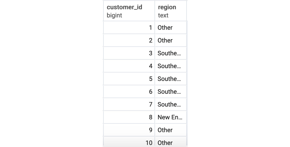
Figure 3.14: Regional query output
In the preceding output, in the case of each customer, a region has been mapped based on the state where the customer resides.
In this exercise, we learned to map various values in a column to other values using the CASE WHEN function.
COALESCE
Another useful technique is to replace NULL values with a standard value. This can be accomplished easily by means of the COALESCE function. COALESCE allows you to list any number of columns and scalar values, and, if the first value in the list is NULL, it will try to fill it in with the second value. The COALESCE function will keep continuing down the list of values until it hits a non-NULL value. If all values in the COALESCE function are NULL, then the function returns NULL.
To illustrate a simple usage of the COALESCE function, let's return to the customers table. Let's say the marketing team would like a list of the first names, last names, and phone numbers of all male customers. However, for those customers with no phone number, they would like the table to instead write the value 'NO PHONE'. We can accomplish this request with COALESCE:
SELECT first_name,
last_name,
COALESCE(phone, 'NO PHONE') as phone
FROM customers
ORDER BY 1;
This query produces the following results:
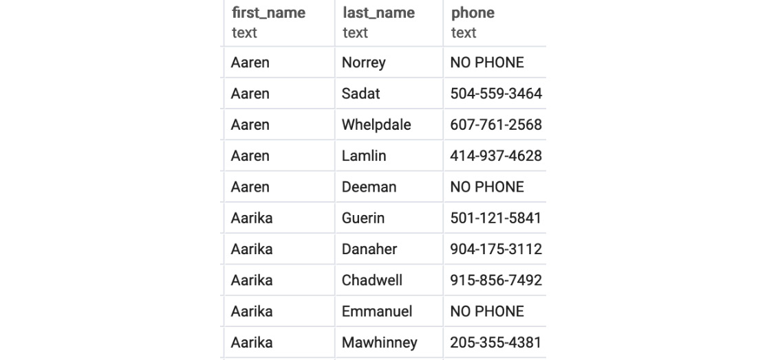
Figure 3.15: Coalesce query
When dealing with creating default values and avoiding NULL, COALESCE will always be helpful.
NULLIF
NULLIF is, in a sense, the opposite of COALESCE. NULLIF is a two-value function and will return NULL if the first value equals the second value.
As an example, imagine that the marketing department has created a new direct mail piece to send to the customer. One of the quirks of this new piece of advertising is that it cannot accept people who have titles longer than three letters.
In our database, the only known title longer than three characters is 'Honorable'. Therefore, they would like you to create a mailing list that is just all the rows with valid street addresses and to blot out all titles with NULL that are spelled as 'Honorable'. This could be done with the following query:
SELECT customer_id,
NULLIF(title, 'Honorable') as title,
first_name,
last_name,
suffix,
email,
gender,
ip_address,
phone,
street_address,
city,
state,
postal_code,
latitude,
longitude,
date_added
FROM customers c
ORDER BY 1
This will blot out all mentions of 'Honorable' from the title column.
LEAST/GREATEST
Two functions that come in handy for data preparation are the LEAST and GREATEST functions. Each function takes any number of values and returns the least or the greatest of the values, respectively.
A simple use of this variable would be to replace the value if it's too high or low. For example, the sales team may want to create a sales list where every scooter is $600 or less than that. We can create this using the following query:
SELECT product_id,
model,
year,
product_type,
LEAST(600.00, base_msrp) as base_msrp,
production_start_date,
production_end_date
FROM products
WHERE product_type='scooter'
ORDER BY 1;
This query will give the following output:
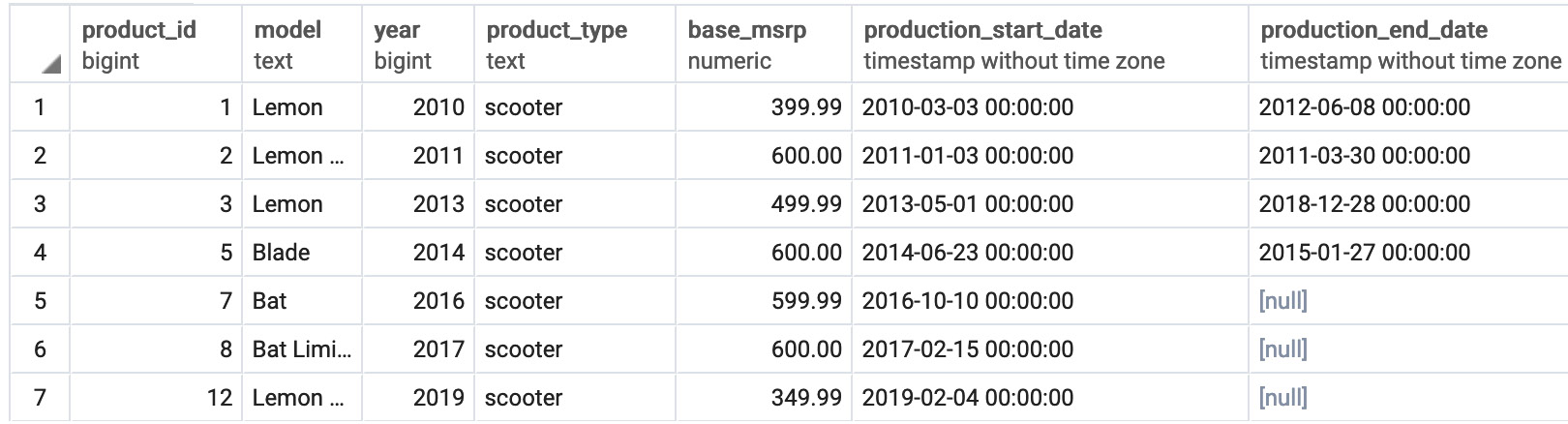
Figure 3.16: Cheaper scooters
Casting
Another useful data transformation is to change the data type of a column within a query. This is usually done to use a function only available to one data type, such as text, while working with a column that is in a different data type, such as a numeric. To change the data type of a column, you simply need to use the column::datatype format, where column is the column name, and datatype is the data type you want to change the column to. For example, to change the year in the products table to a text column in a query, use the following query:
SELECT product_id,
model,
year::TEXT,
product_type,
base_msrp,
production_start_date,
production_end_date
FROM products;
This will convert the year column to text. You can now apply text functions to this transformed column. There is one final catch; not every data type can be cast to a specific data type. For instance, datetime cannot be cast to float types. Your SQL client will throw an error if you ever make an unexpected strange conversion.
DISTINCT and DISTINCT ON
Often, when looking through a dataset, you may be interested in determining the unique values in a column or group of columns. This is the primary use case of the DISTINCT keyword. For example, if you wanted to know all the unique model years in the products table, you could use the following query:
SELECT DISTINCT year
FROM products
ORDER BY 1;
This gives the following result:

Figure 3.17: Distinct model years
You can also use it with multiple columns to get all distinct column combinations present. For example, to find all distinct years and what product types were released for those model years, you can simply use the following:
SELECT DISTINCT year, product_type
FROM products
ORDER BY 1, 2;
This gives the following output:

Figure 3.18: Distinct model years and product types
A keyword related to DISTINCT is DISTINCT ON. DISTINCT ON allows you to ensure that only one row is returned where one or more columns are always unique in the set. The general syntax of a DISTINCT ON query is:
SELECT DISTINCT ON (distinct_column)
column_1,
column_2,
…
column_n
FROM table
ORDER BY order_column;
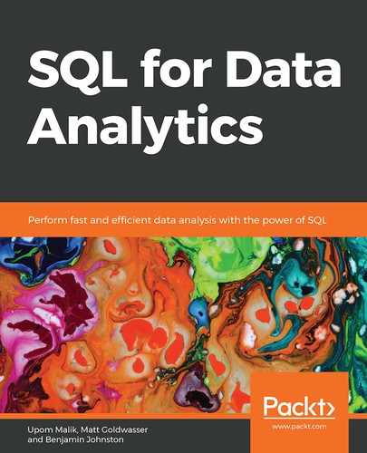
Here, dictinct_column is the column or columns you want to be distinct in your query, column_1 through column_n are the columns you want in the query, and order_column allows you to determine the first row that will be returned for a DISTINCT ON query if multiple columns have the same value for distinct_column. For order_column, the first column mentioned should be distinct_column. If an ORDER BY clause is not specified, the first row will be decided randomly. To clarify, let's say you wanted to get a unique list of salespeople where each salesperson has a unique first name. In the case that two salespeople have the same first name, we will return the one that started earlier. This query would look like this:
SELECT DISTINCT ON (first_name)
*
FROM salespeople
ORDER BY first_name, hire_date;
It will return the following:
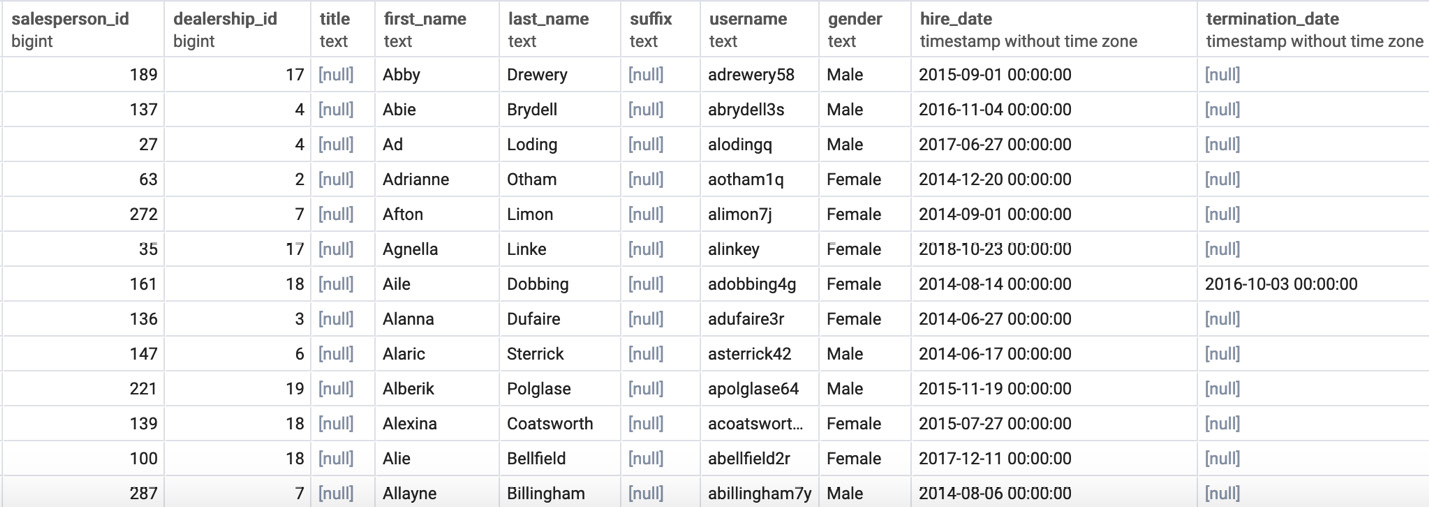
Figure 3.19: DISTINCT ON first_name
This table now guarantees that every row has a distinct username and that the row returned if multiple users have a given first name is the person hired there with that first name. For example, if the salespeople table has multiple rows with the first name 'Abby', the row seen in Figure 3.19 with the name 'Abby' (the first row in the outputs) was for the first person employed at the company with the name 'Abby'.
Activity 5: Building a Sales Model Using SQL Techniques
The aim of this activity is to clean and prepare our data for analysis using SQL techniques. The data science team wants to build a new model to help predict which customers are the best prospects for remarketing. A new data scientist has joined their team and does not know the database well enough to pull a dataset for this new model. The responsibility has fallen to you to help the new data scientist prepare and build a dataset to be used to train a model. Write a query to assemble a dataset that will do the following:
- Open a SQL client and connect to the database.
- Use INNER JOIN to join the customers table to the sales table.
- Use INNER JOIN to join the products table to the sales table.
- Use LEFT JOIN to join the dealerships table to the sales table.
- Now, return all columns of the customers table and the products table.
- Then, return the dealership_id column from the sales table, but fill in dealership_id in sales with -1 if it is NULL.
- Add a column called high_savings that returns 1 if the sales amount was 500 less than base_msrp or lower. Otherwise, it returns 0.
Expected Output:

Figure 3.20: Building a sales model query
Note
The solution for the activity can be found on page 321.
Summary
SQL provides us with many tools for mixing and cleaning data. We have learned how joins allow users to combine multiple tables, while UNION and subqueries allow us to combine multiple queries. We have also learned how SQL has a wide variety of functions and keywords that allow users to map new data, fill in missing data, and remove duplicate data. Keywords such as CASE WHEN, COALESCE, NULLIF, and DISTINCT allow us to make changes to data quickly and easily.
Now that we know how to prepare a dataset, we will learn how to start making analytical insights in the next chapter using aggregates.