Chapter 9

Using SQL to Uncover the Truth – a Case Study

Learning Objectives

By the end of this chapter, you will be able to:

• Use the scientific method and critical thinking to glean insights about your data
• Solve real-world problems outside of those described within this book by using the skills that you have acquired
• Convert data and hypotheses into actionable tasks and insights
• Use the skills developed in this book to solve problems in your specific problem domain

In this chapter, we will examine an extensive and detailed real-world case study of sales data. This case study will not only demonstrate the processes used in SQL analysis to find solutions for actual problems but will also provide you with confidence and experience in solving such problems.

Introduction

Throughout SQL for Data Analytics, you have learned a range of new skills, including basic descriptive statistics, SQL commands and importing and exporting data in PostgreSQL, as well as more advanced methods, such as functions and triggers. In this final chapter of the book, we will combine these new skills with the scientific method and critical thinking to solve the real-world problem of understanding the cause of an unexpected drop in sales. This chapter provides a case study and will help you to develop confidence in applying your new SQL skillset to your own problem domains. To solve the problem presented in this use case, we will use the complete range of your newly developed skills, from using basic SQL searches to filter out the available information to aggregating and joining multiple sets of information and using windowing methods to group the data in a logical manner. By completing case studies such as this, you will refine one of the key tools in your data analysis toolkit, providing a boost to your data science career.

Case Study

Throughout this chapter, we will cover the following case study. The new ZoomZoom Bat Scooter is now available for sale exclusively through its website. Sales are looking good, but suddenly, pre-orders start plunging by 20% after a couple of weeks. What's going on? As the best data analyst at ZoomZoom, it's been assigned to you to figure it out.

Scientific Method

In this case study, we will be following the scientific method to help solve our problem, which, at its heart, is about testing guesses (or hypotheses) using objectively collected data. We can decompose the scientific method into the following key steps:

1. Define the question to answer what caused the drop-in sales of the Bat Scooter after approximately 2 weeks.
2. Complete background research to gather sufficient information to propose an initial hypothesis for the event or phenomenon.
3. Construct a hypothesis to explain the event or answer the question.
4. Define and execute an objective experiment to test the hypothesis. In an ideal scenario, all aspects of the experiment should be controlled and fixed, except for the phenomenon that is being tested under the hypothesis.
5. Analyze the data collected during the experiment.
6. Report the result of the analysis, which will hopefully explain why there was a drop in the sale of Bat Scooters.

It is to be noted that in this chapter, we are completing a post-hoc analysis of the data, that is, the event has happened, and all available data has been collected. Post-hoc data analysis is particularly useful when events have been recorded that cannot be repeated or when certain external factors cannot be controlled. It is with this data that we are able to perform our analysis, and, as such, we will extract information to support or refute our hypothesis. We will, however, be unable to definitively confirm or reject the hypothesis without practical experimentation. The question that will be the subject of this chapter and that we need to answer is this: why did the sales of the ZoomZoom Bat Scooter drop by approximately 20% after about 2 weeks?

So, let's start with the absolute basics.

Exercise 34: Preliminary Data Collection Using SQL Techniques

In this exercise, we will collect preliminary data using SQL techniques. We have been told that the pre-orders for the ZoomZoom Bat Scooter were good, but the orders suddenly dropped by 20%. So, when was production started on the scooter, and how much was it selling for? How does the Bat Scooter compare with other types of scooters in terms of price? The goal of this exercise is to answer these questions:

1. Load the sqlda database from the accompanying source code located at https://github.com/TrainingByPackt/SQL-for-Data-Analytics/tree/master/Datasets:

   $ psql sqlda

2. List the model, base_msrp (MSRP: manufacturer's suggested retail price) and production_start_date fields within the product table for product types matching scooter:

   sqlda=# SELECT model, base_msrp, production_start_date FROM products WHERE product_type='scooter';

   The following table shows the details of all the products for the scooter product type:

   

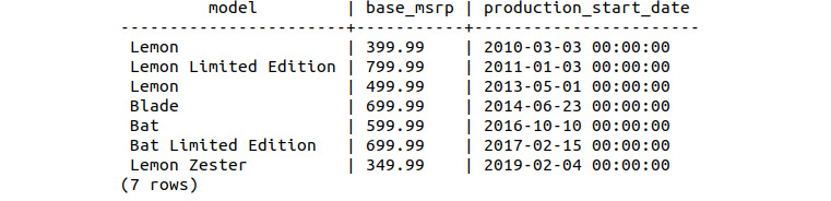
   Figure 9.1: Basic list of scooters with a base manufacturer suggesting a retail price and production date

   Looking at the results from the search, we can see that we have two scooter products with Bat in the name; Bat and Bat Limited Edition. The Bat Scooter, which started production on October 10, 2016, with a suggested retail price of $599.99; and the Bat Limited Edition Scooter, which started production approximately 4 months later, on February 15, 2017, at a price of $699.99.

   Looking at the product information supplied, we can see that the Bat Scooter is somewhat unique from a price perspective, being the only scooter with a suggested retail price of $599.99. There are two others at $699.99 and one at $499.99.

   Similarly, if we consider the production start date in isolation, the original Bat Scooter is again unique in that it is the only scooter starting production in the last quarter or even half of the year (date format: YYYY-MM-DD). All other scooters start production in the first half of the year, with only the Blade scooter starting production in June.

   In order to use the sales information in conjunction with the product information available, we also need to get the product ID for each of the scooters.

3. Extract the model name and product IDs for the scooters available within the database. We will need this information to reconcile the product information with the available sales information:

   sqlda=# SELECT model, product_id FROM products WHERE product_type='scooter';

   The query yields the product IDs shown in the following table:

   

   Figure 9.2: Scooter product ID codes

4. Insert the results of this query into a new table called product_names:

   sqlda=# SELECT model, product_id INTO product_names FROM products WHERE product_type='scooter';

   Inspect the contents of the product_names table shown in the following figure:

Figure 9.3: Contents of the new product_names table

As described in the output, we can see that the Bat Scooter lies between the price points of some of the other scooters and that it was also manufactured a lot later in the year compared to the others.

By completing this very preliminary data collection step, we have the information required to collect sales data on the Bat Scooter as well as other scooter products for comparison. While this exercise involved using the simplest SQL commands, it has already yielded some useful information.

This exercise has also demonstrated that even the simplest SQL commands can reveal useful information and that they should not be underestimated. In the next exercise, we will try to extract the sales information related to the reduction in sales of the Bat Scooter.

Exercise 35: Extracting the Sales Information

In this exercise, we will use a combination of simple SELECT statements, as well as aggregate and window functions, to examine the sales data. With the preliminary information at hand, we can use it to extract the Bat Scooter sales records and discover what is actually going on. We have a table, product_names, that contains both the model names and product IDs. We will need to combine this information with the sales records and extract only those for the Bat Scooter:

1. Load the sqlda database:

   $ psql sqlda

2. List the available fields in the sqlda database:

   sqlda=# d

   The preceding query yields the following fields present in the database:

   

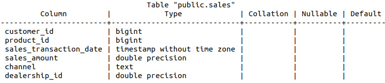
   Figure 9.4: Structure of the sales table

   We can see that we have references to customer and product IDs, as well as the transaction date, sales information, the sales channel, and the dealership ID.

3. Use an inner join on the product_id columns of both the product_names table and the sales table. From the result of the inner join, select the model, customer_id, sales_transaction_date, sales_amount, channel, and dealership_id, and store the values in a separate table called product_sales:

   sqlda=# SELECT model, customer_id, sales_transaction_date, sales_amount, channel, dealership_id INTO products_sales FROM sales INNER JOIN product_names ON sales.product_id=product_names.product_id;

   The output of the preceding code can be seen in the next step.

   Note

   Throughout this chapter, we will be storing the results of queries and calculations in separate tables as this will allow you to look at the results of the individual steps in the analysis at any time. In a commercial/production setting, we would typically only store the end result in a separate table, depending upon the context of the problem being solved.

4. Look at the first five rows of this new table by using the following query:

   sqlda=# SELECT * FROM products_sales LIMIT 5;

   The following table lists the top five customers who made a purchase. It shows the sale amount and the transaction details, such as the date and time:

   

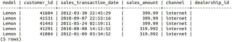
   Figure 9.5: The combined product sales table

5. Select all the information from the product_sales table that is available for the Bat Scooter and order the sales information by sales_transaction_date in ascending order. By selecting the data in this way, we can look at the first few days of the sales records in detail:

   sqlda=# SELECT * FROM products_sales WHERE model='Bat' ORDER BY sales_transaction_date;

   The preceding query generates the following output:

   

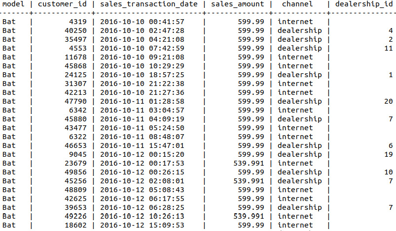
   Figure 9.6: Ordered sales records

6. Count the number of records available by using the following query:

   sqlda=# SELECT COUNT(model) FROM products_sales WHERE model='Bat';

   The model count for the 'Bat' model is as shown here:

   

   Figure 9.7: Count of the number of sales records

   So, we have 7328 sales, beginning October 10, 2016. Check the date of the final sales record by performing the next step.

7. Determine the last sale date for the Bat Scooter by selecting the maximum (using the MAX function) for sales_transaction_date:

   sqlda=# SELECT MAX(sales_transaction_date) FROM products_sales WHERE model='Bat';

   The last sale date is shown here:

   

   Figure 9.8: Last sale date

   The last sale in the database occurred on May 31, 2019.

8. Collect the daily sales volume for the Bat Scooter and place it in a new table called bat_sales to confirm the information provided by the sales team stating that sales dropped by 20% after the first 2 weeks:

   sqlda=# SELECT * INTO bat_sales FROM products_sales WHERE model='Bat' ORDER BY sales_transaction_date;

9. Remove the time information to allow tracking of sales by date, since, at this stage, we are not interested in the time at which each sale occurred. To do so, run the following query:

   sqlda=# UPDATE bat_sales SET sales_transaction_date=DATE(sales_transaction_date);

10. Display the first five records of bat_sales ordered by sales_transaction_date:

    sqlda=# SELECT * FROM bat_sales ORDER BY sales_transaction_date LIMIT 5;

    The following is the output of the preceding code:

    

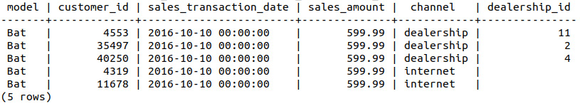
    Figure 9.9: First five records of Bat Scooter sales

11. Create a new table (bat_sales_daily) containing the sales transaction dates and a daily count of total sales:

    sqlda=# SELECT sales_transaction_date, COUNT(sales_transaction_date) INTO bat_sales_daily FROM bat_sales GROUP BY sales_transaction_date ORDER BY sales_transaction_date;

12. Examine the first 22 records (a little over 3 weeks), as sales were reported to have dropped after approximately the first 2 weeks:

    sqlda=# SELECT * FROM bat_sales_daily LIMIT 22;

    This will display the following output:

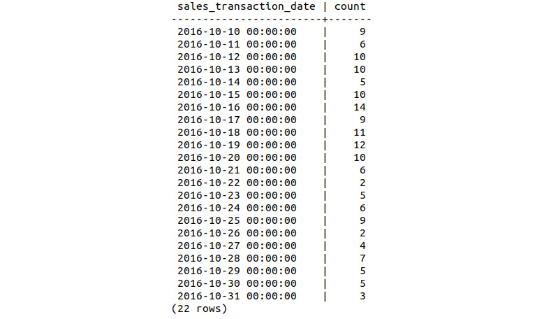
Figure 9.10: First 3 weeks of sales

We can see a drop-in sales after October 20, as there are 7 days in the first 11 rows that record double-digit sales, and none over the next 11 days.

At this stage, we can confirm that there has been a drop off in sales, although we are yet to quantify precisely the extent of the reduction or the reason for the drop off in sales.

Activity 18: Quantifying the Sales Drop

In this activity, we will use our knowledge of the windowing methods that we learned in Chapter 5, Window Functions for Data Analysis. In the previous exercise, we identified the occurrence of the sales drop as being approximately 10 days after launch. Here, we will try to quantify the drop off in sales for the Bat Scooter.

Perform the following steps to complete the activity:

1. Load the sqlda database from the accompanying source code located at https://github.com/TrainingByPackt/SQL-for-Data-Analytics/tree/master/Datasets.
2. Using the OVER and ORDER BY statements, compute the daily cumulative sum of sales. This provides us with a discrete count of sales over time on a daily basis. Insert the results into a new table called bat_sales_growth.
3. Compute a 7-day lag of the sum column, and then insert all the columns of bat_sales_daily and the new lag column into a new table, bat_sales_daily_delay. This lag column indicates what sales were like 1 week prior to the given record, allowing us to compare sales with the previous week.
4. Inspect the first 15 rows of bat_sales_growth.
5. Compute the sales growth as a percentage, comparing the current sales volume to that of 1 week prior. Insert the resulting table into a new table called bat_sales_delay_vol.
6. Compare the first 22 values of the bat_sales_delay_vol table to ascertain a sales drop.

Expected Output

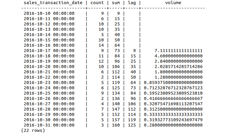
Figure 9.11: Relative sales volume of the Bat Scooter over 3 weeks

Note

The solution to the activity can be found on page 354.

While the count and cumulative sum columns are reasonably straightforward, why do we need the lag and volume columns? This is because we are looking for drops in sales growth over the first couple of weeks, hence, we compare the daily sum of sales to the same values 7 days earlier (the lag). By subtracting the sum and lag values and dividing by the lag, we obtain the volume value and can determine sales growth compared to the previous week.

Notice that the sales volume on October 17 is 700% above that of the launch date of October 10. By October 22, the volume is over double that of the week prior. As time passes, this relative difference begins to decrease dramatically. By the end of October, the volume is 28% higher than the week prior. At this stage, we have observed and confirmed the presence of a reduction in sales growth after the first 2 weeks. The next stage is to attempt to explain the causes of the reduction.

Exercise 36: Launch Timing Analysis

In this exercise, we will try to identify the causes of a sales drop. Now that we have confirmed the presence of the sales growth drop, we will try to explain the cause of the event. We will test the hypothesis that the timing of the scooter launch attributed to the reduction in sales. Remember, in Exercise 34, Preliminary Data Collection Using SQL Techniques, that the ZoomZoom Bat Scooter launched on October 10, 2016. Observe the following steps to complete the exercise:

1. Load the sqlda database:

   $ psql sqlda

2. Examine the other products in the database. In order to determine whether the launch date attributed to the sales drop, we need to compare the ZoomZoom Bat Scooter to other scooter products according to the launch date. Execute the following query to check the launch dates:

   sqlda=# SELECT * FROM products;

   The following figure shows the launch dates for all the products:

   

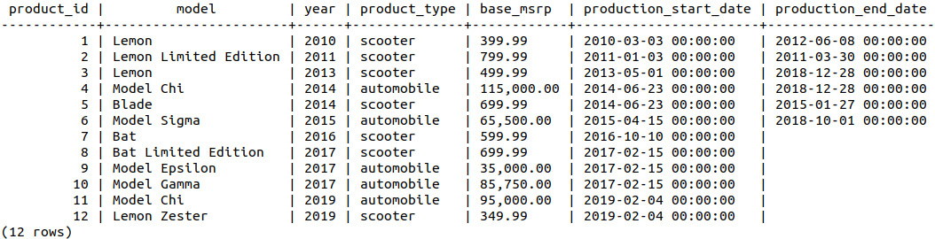
   Figure 9.12: Products with launch dates

   All the other products launched before July, compared to the Bat Scooter, which launched in October.

3. List all scooters from the products table, as we are only interested in comparing scooters:

   sqlda=# SELECT * FROM products WHERE product_type='scooter';

   The following table shows all the information for products with the product type of scooter:

   

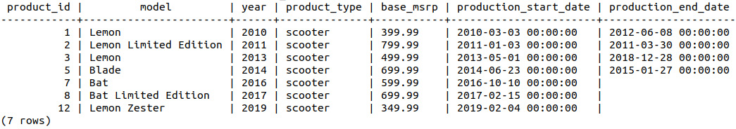
   Figure 9.13: Scooter product launch dates

   To test the hypothesis that the time of year had an impact on sales performance, we require a scooter model to use as the control or reference group. In an ideal world, we could launch the ZoomZoom Bat Scooter in a different location or region, for example, but just at a different time, and then compare the two. However, we cannot do this here. Instead, we will choose a similar scooter launched at a different time. There are several different options in the product database, each with its own similarities and differences to the experimental group (ZoomZoom Bat Scooter). In our opinion, the Bat Limited Edition Scooter is suitable for comparison (the control group). It is slightly more expensive, but it was launched only 4 months after the Bat Scooter. Looking at its name, the Bat Limited Edition Scooter seems to share most of the same features, with a number of extras given that it's a "limited edition."

4. Select the first five rows of the sales database:

   sqlda=# SELECT * FROM sales LIMIT 5;

   The sales information for the first five customers is as follows:

   

   Figure 9.14: First five rows of sales data

5. Select the model and sales_transaction_date columns from both the products and sales tables for the Bat Limited Edition Scooter. Store the results in a table, bat_ltd_sales, ordered by the sales_transaction_date column, from the earliest date to the latest:

   sqlda=# SELECT products.model, sales.sales_transaction_date INTO bat_ltd_sales FROM sales INNER JOIN products ON sales.product_id=products.product_id WHERE sales.product_id=8 ORDER BY sales.sales_transaction_date;

6. Select the first five lines of bat_ltd_sales, using the following query:

   sqlda=# SELECT * FROM bat_ltd_sales LIMIT 5;

   The following table shows the transaction details for the first five entries of Bat Limited Edition:

   

   Figure 9.15: First five sales of the Bat Limited Edition Scooter

7. Calculate the total number of sales for Bat Limited Edition. We can check this by using the COUNT function:

   sqlda=# SELECT COUNT(model) FROM bat_ltd_sales;

   The total sales count can be seen in the following figure:

   

   Figure 9.16: Count of Bat Limited Edition sales

   This is compared to the original Bat Scooter, which sold 7,328 items.

8. Check the transaction details of the last Bat Limited Edition sale. We can check this by using the MAX function:

   sqlda=# SELECT MAX(sales_transaction_date) FROM bat_ltd_sales;

   The transaction details of the last Bat Limited Edition product are as follows:

   

   Figure 9.17: Last date (MAX) of the Bat Limited Edition sale

9. Adjust the table to cast the transaction date column as a date, discarding the time information. As with the original Bat Scooter, we are only interested in the date of the sale, not the date and time of the sale. Write the following query:

   sqlda=# ALTER TABLE bat_ltd_sales ALTER COLUMN sales_transaction_date TYPE date;

10. Again, select the first five records of bat_ltd_sales:

    sqlda=# SELECT * FROM bat_ltd_sales LIMIT 5;

    The following table shows the first five records of bat_ltd_sales:

    

    Figure 9.18: Select the first five Bat Limited Edition sales by date

11. In a similar manner to the standard Bat Scooter, create a count of sales on a daily basis. Insert the results into the bat_ltd_sales_count table by using the following query:

    sqlda=# SELECT sales_transaction_date, count(sales_transaction_date) INTO bat_ltd_sales_count FROM bat_ltd_sales GROUP BY sales_transaction_date ORDER BY sales_transaction_date;

12. List the sales count of all the Bat Limited products using the following query:

    sqlda=# SELECT * FROM bat_ltd_sales_count;

    The sales count is shown in the following figure:

    

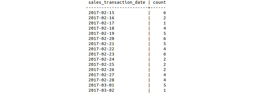
    Figure 9.19: Bat Limited Edition daily sales

13. Compute the cumulative sum of the daily sales figures and insert the resulting table into bat_ltd_sales_growth:

    sqlda=# SELECT *, sum(count) OVER (ORDER BY sales_transaction_date) INTO bat_ltd_sales_growth FROM bat_ltd_sales_count;

14. Select the first 22 days of sales records from bat_ltd_sales_growth:

    sqlda=# SELECT * FROM bat_ltd_sales_growth LIMIT 22;

    The following table displays the first 22 records of sales growth:

    

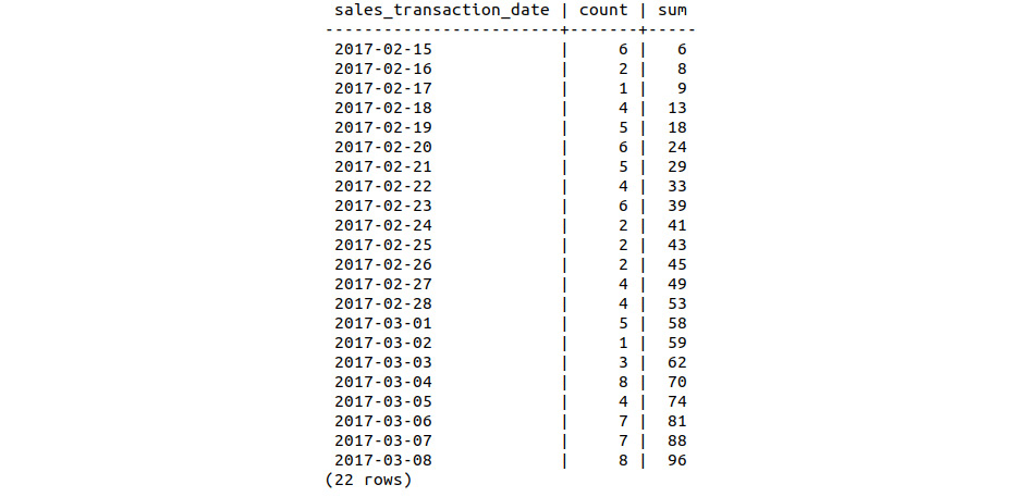
    Figure 9.20: Bat Limited Edition sales – cumulative sum

15. Compare this sales record with the one for the original Bat Scooter sales, as shown in the following code:

    sqlda=# SELECT * FROM bat_sales_growth LIMIT 22;

    The following table shows the sales details for the first 22 records of the bat_sales_growth table:

    

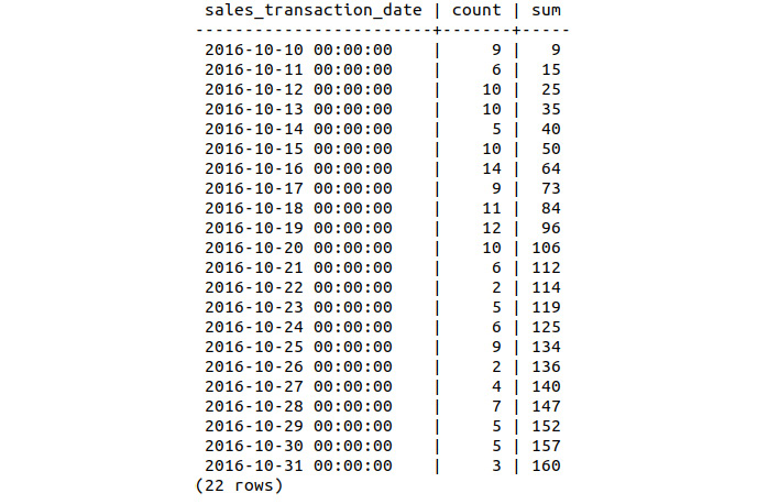
    Figure 9.21: Bat Scooter cumulative sales for 22 rows

    Sales of the limited-edition scooter did not reach double digits during the first 22 days, nor did the daily volume of sales fluctuate as much. In keeping with the overall sales figure, the limited edition sold 64 fewer units over the first 22 days.

16. Compute the 7-day lag function for the sum column and insert the results into the bat_ltd_sales_delay table:

    sqlda=# SELECT *, lag(sum , 7) OVER (ORDER BY sales_transaction_date) INTO bat_ltd_sales_delay FROM bat_ltd_sales_growth;

17. Compute the sales growth for bat_ltd_sales_delay in a similar manner to the exercise completed in Activity 18, Quantifying the Sales Drop. Label the column for the results of this calculation as volume and store the resulting table in bat_ltd_sales_vol:

    sqlda=# SELECT *, (sum-lag)/lag AS volume INTO bat_ltd_sales_vol FROM bat_ltd_sales_delay;

18. Look at the first 22 records of sales in bat_ltd_sales_vol:

    sqlda=# SELECT * FROM bat-ltd_sales_vol LIMIT 22;

    The sales volume can be seen in the following figure:

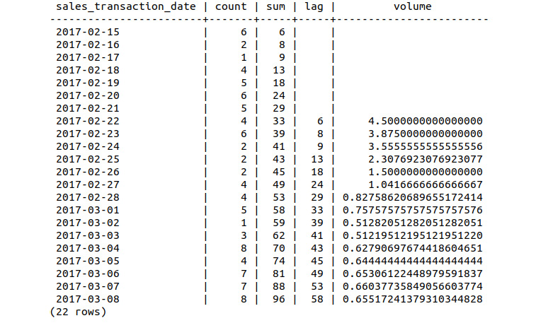
Figure 9.22: Bat Scooter cumulative sales showing volume

Looking at the volume column in the preceding diagram, we can again see that the sales growth is more consistent than the original Bat Scooter. The growth within the first week is less than that of the original model, but it is sustained over a longer period. After 22 days of sales, the sales growth of the limited-edition scooter is 65% compared to the previous week, as compared with the 28% growth identified in the second activity of the chapter.

At this stage, we have collected data from two similar products launched at different time periods and found some differences in the trajectory of the sales growth over the first 3 weeks of sales. In a professional setting, we may also consider employing more sophisticated statistical comparison methods, such as tests for differences of mean, variance, survival analysis, or other techniques. These methods lie outside the scope of this book and, as such, limited comparative methods will be used.

While we have shown there to be a difference in sales between the two Bat Scooters, we also cannot rule out the fact that the sales differences can be attributed to the difference in the sales price of the two scooters, with the limited-edition scooter being $100 more expensive. In the next activity, we will compare the sales of the Bat Scooter to the 2013 Lemon, which is $100 cheaper, was launched 3 years prior, is no longer in production, and started production in the first half of the calendar year.

Activity 19: Analyzing the Difference in the Sales Price Hypothesis

In this activity, we are going to investigate the hypothesis that the reduction in sales growth can be attributed to the price point of the Bat Scooter. Previously, we considered the launch date. However, there could be another factor – the sales price included. If we consider the product list of scooters shown in Figure 9.23, and exclude the Bat model scooter, we can see that there are two price categories, $699.99 and above, or $499.99 and below. The Bat Scooter sits exactly between these two groups; perhaps the reduction in sales growth can be attributed to the different pricing model. In this activity, we will test this hypothesis by comparing Bat sales to the 2013 Lemon:

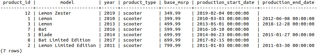
Figure 9.23: List of scooter models

The following are the steps to perform:

1. Load the sqlda database from the accompanying source code located at https://github.com/TrainingByPackt/SQL-for-Data-Analytics/tree/master/Datasets.
2. Select the sales_transaction_date column from the year 2013 for Lemon model sales and insert the column into a table called lemon_sales.
3. Count the sales records available for 2013 for the Lemon model.
4. Display the latest sales_transaction_date column.
5. Convert the sales_transaction_date column to a date type.
6. Count the number of sales per day within the lemon_sales table and insert the data into a table called lemon_sales_count.
7. Calculate the cumulative sum of sales and insert the corresponding table into a new table labeled lemon_sales_sum.
8. Compute the 7-day lag function on the sum column and save the result to lemon_sales_delay.
9. Calculate the growth rate using the data from lemon_sales_delay and store the resulting table in lemon_sales_growth.
10. Inspect the first 22 records of the lemon_sales_growth table by examining the volume data.

Expected Output

Figure 9.24: Sales growth of the Lemon Scooter

Note

The solution to the activity can be found on page 356.

Now that we have collected data to test the two hypotheses of timing and cost, what observations can we make and what conclusions can we draw? The first observation that we can make is regarding the total volume of sales for the three different scooter products. The Lemon Scooter, over its production life cycle of 4.5 years, sold 16,558 units, while the two Bat Scooters, the Original and Limited Edition models, sold 7,328 and 5,803 units, respectively, and are still currently in production, with the Bat Scooter launching about 4 months earlier and with approximately 2.5 years of sales data available. Looking at the sales growth of the three different scooters, we can also make a few different observations:

• The original Bat Scooter, which launched in October at a price of $599.99, experienced a 700% sales growth in its second week of production and finished the first 22 days with 28% growth and a sales figure of 160 units.
• The Bat Limited Edition Scooter, which launched in February at a price of $699.99, experienced 450% growth at the start of its second week of production and finished with 96 sales and 66% growth over the first 22 days.
• The 2013 Lemon Scooter, which launched in May at a price of $499.99, experienced 830% growth in the second week of production and ended its first 22 days with 141 sales and 55% growth.

Based on this information, we can make a number of different conclusions:

• The initial growth rate starting in the second week of sales correlates to the cost of the scooter. As the cost increased to $699.99, the initial growth rate dropped from 830% to 450%.
• The number of units sold in the first 22 days does not directly correlate to the cost. The $599.99 Bat Scooter sold more than the 2013 Lemon Scooter in that first period despite the price difference.
• There is some evidence to suggest that the reduction in sales can be attributed to seasonal variations given the significant reduction in growth and the fact that the original Bat Scooter is the only one released in October. So far, the evidence suggests that the drop can be attributed to the difference in launch timing.

Before we draw the conclusion that the difference can be attributed to seasonal variations and launch timing, let's ensure that we have extensively tested a range of possibilities. Perhaps marketing work, such as email campaigns, that is, when the emails were sent, and the frequency with which the emails were opened, made a difference.

Now that we have considered both the launch timing and the suggested retail price of the scooter as a possible cause of the reduction in sales, we will direct our efforts to other potential causes, such as the rate of opening of marketing emails. Does the marketing email opening rate have an effect on sales growth throughout the first 3 weeks? We will find this out in our next exercise.

Exercise 37: Analyzing Sales Growth by Email Opening Rate

In this exercise, we will analyze the sales growth using the email opening rate. To investigate the hypothesis that a decrease in the rate of opening emails impacted the Bat Scooter sales rate, we will again select the Bat and Lemon Scooters and will compare the email opening rate.

Perform the following steps to complete the exercise:

1. Load the sqlda database:

   $ psql sqlda

2. Firstly, look at the emails table to see what information is available. Select the first five rows of the emails table:

   sqlda=# SELECT * FROM emails LIMIT 5;

   The following table displays the email information for the first five rows:

   

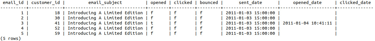
   Figure 9.25: Sales growth of the Lemon Scooter

   To investigate our hypothesis, we need to know whether an email was opened, and when it was opened, as well as who the customer was who opened the email and whether that customer purchased a scooter. If the email marketing campaign was successful in maintaining the sales growth rate, we would expect a customer to open an email soon before a scooter was purchased.

   The period in which the emails were sent, as well as the ID of customers who received and opened an email, can help us to determine whether a customer who made a sale may have been encouraged to do so following the receipt of an email.

3. To determine the hypothesis, we need to collect the customer_id column from both the emails table and the bat_sales table for the Bat Scooter, the opened, sent_date, opened_date, and email_subject columns from emails table, as well as the sales_transaction_date column from the bat_sales table. As we only want the email records of customers who purchased a Bat Scooter, we will join the customer_id column in both tables. Then, insert the results into a new table – bat_emails:

   sqlda=# SELECT emails.email_subject, emails.customer_id, emails.opened, emails.sent_date, emails.opened_date, bat_sales.sales_transaction_date INTO bat_emails FROM emails INNER JOIN bat_sales ON bat_sales.customer_id=emails.customer_id ORDER BY bat_sales.sales_transaction_date;

4. Select the first 10 rows of the bat_emails table, ordering the results by sales_transaction_date:

   sqlda=# SELECT * FROM bat_emails LIMIT 10;

   The following table shows the first 10 rows of the bat_emails table ordered by sales_transaction_date:

   

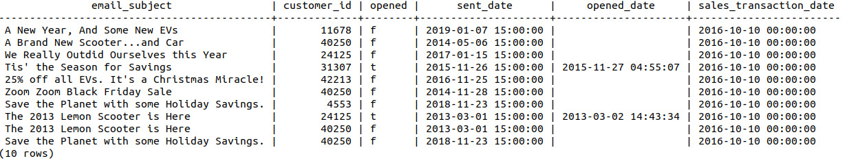
   Figure 9.26: Email and sales information joined on customer_id

   We can see here that there are several emails unopened, over a range of sent dates, and that some customers have received multiple emails. Looking at the subjects of the emails, some of them don't seem related to the Zoom scooters at all.

5. Select all rows where the sent_date email predates the sales_transaction_date column, order by customer_id, and limit the output to the first 22 rows. This will help us to know which emails were sent to each customer before they purchased their scooter. Write the following query to do so:

   sqlda=# SELECT * FROM bat_emails WHERE sent_date < sales_transaction_date ORDER BY customer_id LIMIT 22;

   The following table lists the emails sent to the customers before the sales_transaction_date column:

   

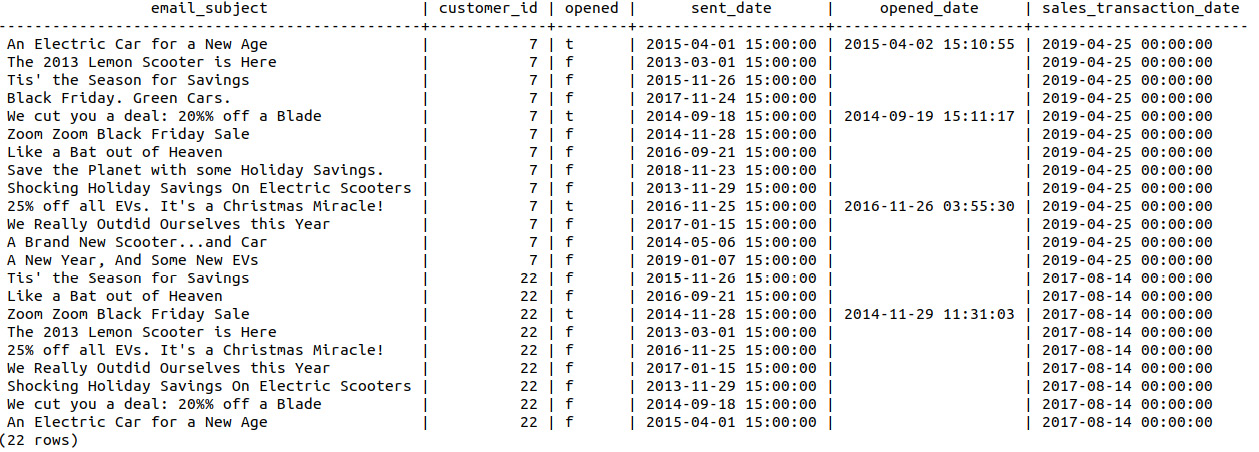
   Figure 9.27: Emails sent to customers before the sale transaction date

6. Delete the rows of the bat_emails table where emails were sent more than 6 months prior to production. As we can see, there are some emails that were sent years before the transaction date. We can easily remove some of the unwanted emails by removing those sent before the Bat Scooter was in production. From the products table, the production start date for the Bat Scooter is October 10, 2016:

   sqlda=# DELETE FROM bat_emails WHERE sent_date < '2016-04-10';

   Note

   In this exercise, we are removing information that we no longer require from an existing table. This differs from the previous exercises, where we created multiple tables each with slightly different information from other. The technique you apply will differ depending upon the requirements of the problem being solved; do you require a traceable record of analysis, or is efficiency and reduced storage key?

7. Delete the rows where the sent date is after the purchase date, as they are not relevant to the sale:

   sqlda=# DELETE FROM bat_emails WHERE sent_date > sales_transaction_date;

8. Delete those rows where the difference between the transaction date and the sent date exceeds 30, as we also only want those emails that were sent shortly before the scooter purchase. An email 1 year beforehand is probably unlikely to influence a purchasing decision, but one closer to the purchase date may have influenced the sales decision. We will set a limit of 1 month (30 days) before the purchase. Write the following query to do so:

   sqlda=# DELETE FROM bat_emails WHERE (sales_transaction_date-sent_date) > '30 days';

9. Examine the first 22 rows again ordered by customer_id by running the following query:

   sqlda=# SELECT * FROM bat_emails ORDER BY customer_id LIMIT 22;

   The following table shows the emails where the difference between the transaction date and the sent date is less than 30:

   

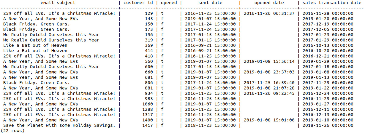
   Figure 9.28: Emails sent close to the date of sale

   At this stage, we have reasonably filtered the available data based on the dates the email was sent and opened. Looking at the preceding email_subject column, it also appears that there are a few emails unrelated to the Bat Scooter, for example, 25% of all EVs. It's a Christmas Miracle! and Black Friday. Green Cars. These emails seem more related to electric car production instead of scooters, and so we can remove them from our analysis.

10. Select the distinct value from the email_subject column to get a list of the different emails sent to the customers:

    sqlda=# SELECT DISTINCT(email_subject) FROM bat_emails;

    The following table shows a list of distinct email subjects:

    

    Figure 9.29: Unique email subjects sent to potential customers of the Bat Scooter

11. Delete all records that have Black Friday in the email subject. These emails do not appear relevant to the sale of the Bat Scooter:

    sqlda=# DELETE FROM bat_emails WHERE position('Black Friday' in email_subject)>0;

    Note

    The position function in the preceding example is used to find any records where the Black Friday string is at the first character in the mail or more in email_structure. Thus, we are deleting any rows where Black Friday is in the email subject. For more information on PostgreSQL, refer to the documentation regarding string functions: https://www.postgresql.org/docs/current/functions-string.html.

12. Delete all rows where 25% off all EVs. It's a Christmas Miracle! and A New Year, And Some New EVs can be found in the email_subject:

    sqlda=# DELETE FROM bat_emails WHERE position('25% off all EV' in email_subject)>0;

    sqlda=# DELETE FROM bat_emails WHERE position('Some New EV' in email_subject)>0;

13. At this stage, we have our final dataset of emails sent to customers. Count the number of rows that are left in the sample by writing the following query:

    sqlda=# SELECT count(sales_transaction_date) FROM bat_emails;

    We can see that 401 rows are left in the sample:

    

    Figure 9.30: Count of the final Bat Scooter email dataset

14. We will now compute the percentage of emails that were opened relative to sales. Count the emails that were opened by writing the following query:

    sqlda=# SELECT count(opened) FROM bat_emails WHERE opened='t'

    We can see that 98 emails were opened:

    

    Figure 9.31: Count of opened Bat Scooter campaign emails

15. Count the customers who received emails and made a purchase. We will determine this by counting the number of unique (or distinct) customers that are in the bat_emails table:

    sqlda=# SELECT COUNT(DISTINCT(customer_id)) FROM bat_emails;

    We can see that 396 customers who received an email made a purchase:

    

    Figure 9.32: Count of unique customers who received a Bat Scooter campaign email

16. Count the unique (or distinct) customers who made a purchase by writing the following query:

    sqlda=# SELECT COUNT(DISTINCT(customer_id)) FROM bat_sales;

    Following is the output of the preceding code:

    

    Figure 9.33: Count of unique customers

17. Calculate the percentage of customers who purchased a Bat Scooter after receiving an email:

    sqlda=# SELECT 396.0/6659.0 AS email_rate;

    The output of the preceding query is displayed as follows:

    

    Figure 9.34: Percentage of customers who received an email

    Note

    In the preceding calculation, you can see that we included a decimal place in the figures, for example, 396.0 instead of a simple integer value (396). This is because the resulting value will be represented as less than 1 percentage point. If we excluded these decimal places, the SQL server would have completed the division operation as integers and the result would be 0.

    Just under 6% of customers who made a purchase received an email regarding the Bat Scooter. Since 18% of customers who received an email made a purchase, there is a strong argument to be made that actively increasing the size of the customer base who receive marketing emails could increase Bat Scooter sales.

18. Limit the scope of our data to be all sales prior to November 1, 2016 and put the data in a new table called bat_emails_threewks. So far, we have examined the email opening rate throughout all available data for the Bat Scooter. Check the rate throughout for the first 3 weeks, where we saw a reduction in sales:

    sqlda=# SELECT * INTO bat_emails_threewks FROM bat_emails WHERE sales_transaction_date < '2016-11-01';

19. Now, count the number of emails opened during this period:

    sqlda=# SELECT COUNT(opened) FROM bat_emails_threewks;

    We can see that we have sent 82 emails during this period:

    

    Figure 9.35: Count of emails opened in the first 3 weeks

20. Now, count the number of emails opened in the first 3 weeks:

    sqlda=# SELECT COUNT(opened) FROM bat_emails_threewks WHERE opened='t';

    The following is the output of the preceding code:

    

    Figure 9.36: Count of emails opened

    We can see that 15 emails were opened in the first 3 weeks.

21. Count the number of customers who received emails during the first 3 weeks of sales and who then made a purchase by using the following query:

    sqlda=# SELECT COUNT(DISTINCT(customer_id)) FROM bat_emails_threewks;

    We can see that 82 customers received emails during the first 3 weeks:

    

    Figure 9.37: Customers who made a purchase in the first 3 weeks

22. Calculate the percentage of customers who opened emails pertaining to the Bat Scooter and then made a purchase in the first 3 weeks by using the following query:

    sqlda=# SELECT 15.0/82.0 AS sale_rate;

    The following table shows the calculated percentage:

    

    Figure 9.38: Percentage of customers in the first 3 weeks who opened emails

    Approximately 18% of customers who received an email about the Bat Scooter made a purchase in the first 3 weeks. This is consistent with the rate for all available data for the Bat Scooter.

23. Calculate how many unique customers we have in total throughout the first 3 weeks. This information is useful context when considering the percentages, we just calculated. 3 sales out of 4 equate to 75% but, in this situation, we would prefer a lower rate of the opening but for a much larger customer base. Information on larger customer bases is generally more useful as it is typically more representative of the entire customer base, rather than a small sample of it. We already know that 82 customers received emails:

    sqlda=# SELECT COUNT(DISTINCT(customer_id)) FROM bat_sales WHERE sales_transaction_date < '2016-11-01';

    The following output reflects 160 customers where the transaction took place before November 1, 2016:

Figure 9.39: Number of distinct customers from bat_sales

There were 160 customers in the first 3 weeks, 82 of whom received emails, which is slightly over 50% of customers. This is much more than 6% of customers over the entire period of availability of the scooter.

Now that we have examined the performance of the email marketing campaign for the Bat Scooter, we need a control or comparison group to establish whether the results were consistent with that of other products. Without a group to compare against, we simply do not know whether the email campaign of the Bat Scooter was good, bad, or neither. We will perform the next exercise to investigate performance.

Exercise 38: Analyzing the Performance of the Email Marketing Campaign

In this exercise, we will investigate the performance of the email marketing campaign for the Lemon Scooter to allow for a comparison with the Bat Scooter. Our hypothesis is that if the email marketing campaign performance of the Bat Scooter is consistent with another, such as the 2013 Lemon, then the reduction in sales cannot be attributed to differences in the email campaigns.

Perform the following steps to complete the exercise:

1. Load the sqlda database:

   $ psql sqlda

2. Drop the existing lemon_sales table:

   sqlda=# DROP TABLE lemon_sales;

3. The 2013 Lemon Scooter is product_id = 3. Select customer_id and sales_transaction_date from the sales table for the 2013 Lemon Scooter. Insert the information into a table called lemon_sales:

   sqlda=# SELECT customer_id, sales_transaction_date INTO lemon_sales FROM sales WHERE product_id=3;

4. Select all information from the emails database for customers who purchased a 2013 Lemon Scooter. Place the information in a new table called lemon_emails:

   sqlda=# SELECT emails.customer_id, emails.email_subject, emails.opened, emails.sent_date, emails.opened_date, lemon_sales.sales_transaction_date INTO lemon_emails FROM emails INNER JOIN lemon_sales ON emails.customer_id=lemon_sales.customer_id;

5. Remove all emails sent before the start of production of the 2013 Lemon Scooter. For this, we first require the date when production started:

   sqlda=# SELECT production_start_date FROM products Where product_id=3;

   The following table shows the production_start_date column:

   

   Figure 9.40: Production start date of the Lemon Scooter

   Now, delete the emails that were sent before the start of production of the 2013 Lemon Scooter:

   sqlda=# DELETE FROM lemon_emails WHERE sent_date < '2013-05-01';

6. Remove all rows where the sent date occurred after the sales_transaction_date column:

   sqlda=# DELETE FROM lemon_emails WHERE sent_date > sales_transaction_date;

7. Remove all rows where the sent date occurred more than 30 days before the sales_transaction_date column:

   sqlda=# DELETE FROM lemon_emails WHERE (sales_transaction_date - sent_date) > '30 days';

8. Remove all rows from lemon_emails where the email subject is not related to a Lemon Scooter. Before doing this, we will search for all distinct emails:

   sqlda=# SELECT DISTINCT(email_subject) FROM lemon_emails;

   The following table shows the distinct email subjects:

   

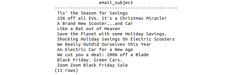
   Figure 9.41: Lemon Scooter campaign emails sent

   Now, delete the email subject not related to the Lemon Scooter using the DELETE command:

   sqlda=# DELETE FROM lemon_emails WHERE POSITION('25% off all EVs.' in email_subject)>0;

   sqlda=# DELETE FROM lemon_emails WHERE POSITION('Like a Bat out of Heaven' in email_subject)>0;

   sqlda=# DELETE FROM lemon_emails WHERE POSITION('Save the Planet' in email_subject)>0;

   sqlda=# DELETE FROM lemon_emails WHERE POSITION('An Electric Car' in email_subject)>0;

   sqlda=# DELETE FROM lemon_emails WHERE POSITION('We cut you a deal' in email_subject)>0;

   sqlda=# DELETE FROM lemon_emails WHERE POSITION('Black Friday. Green Cars.' in email_subject)>0;

   sqlda=# DELETE FROM lemon_emails WHERE POSITION('Zoom' in email_subject)>0;

9. Now, check how many emails of lemon_scooter customers were opened:

   sqlda=# SELECT COUNT(opened) FROM lemon_emails WHERE opened='t';

   We can see that 128 emails were opened:

   

   Figure 9.42: Lemon Scooter campaign emails opened

10. List the number of customers who received emails and made a purchase:

    sqlda=# SELECT COUNT(DISTINCT(customer_id)) FROM lemon_emails;

    The following figure shows that 506 customers made a purchase after receiving emails:

    

    Figure 9.43: Unique customers who purchased a Lemon Scooter

11. Calculate the percentage of customers who opened the received emails and made a purchase:

    sqlda=# SELECT 128.0/506.0 AS email_rate;

    We can see that 25% of customers opened the emails and made a purchase:

    

    Figure 9.44: Lemon Scooter customer email rate

12. Calculate the number of unique customers who made a purchase:

    sqlda=# SELECT COUNT(DISTINCT(customer_id)) FROM lemon_sales;

    We can see that 13854 customers made a purchase:

    

    Figure 9.45: Count of unique Lemon Scooter customers

13. Calculate the percentage of customers who made a purchase having received an email. This will enable a comparison with the corresponding figure for the Bat Scooter:

    sqlda=# SELECT 506.0/13854.0 AS email_sales;

    The preceding calculation generates a 36% output:

    

    Figure 9.46: Lemon Scooter customers who received an email

14. Select all records from lemon_emails where a sale occurred within the first 3 weeks of the start of production. Store the results in a new table – lemon_emails_threewks:

    sqlda=# SELECT * INTO lemon_emails_threewks FROM lemon_emails WHERE sales_transaction_date < '2013-06-01';

15. Count the number of emails that were made for Lemon Scooters in the first 3 weeks:

    sqlda=# SELECT COUNT(sales_transaction_date) FROM lemon_emails_threewks;

    The following is the output of the preceding code:

Figure 9.47: Unique sales of the Lemon Scooter in the first 3 weeks

There is a lot of interesting information here. We can see that 25% of customers who opened an email made a purchase, which is a lot higher than the 18% figure for the Bat Scooter. We have also calculated that just over 3.6% of customers who purchased a Lemon Scooter were sent an email, which is much lower than the almost 6% of Bat Scooter customers. The final interesting piece of information we can see is that none of the Lemon Scooter customers received an email during the first 3 weeks of product launch compared with the 82 Bat Scooter customers, which is approximately 50% of all customers in the first 3 weeks!

In this exercise, we investigated the performance of an email marketing campaign for the Lemon Scooter to allow for a comparison with the Bat Scooter using various SQL techniques.

Conclusions

Now that we have collected a range of information about the timing of the product launches, the sales prices of the products, and the marketing campaigns, we can make some conclusions regarding our hypotheses:

• In Exercise 36, Launch Timing Analysis, we gathered some evidence to suggest that launch timing could be related to the reduction in sales after the first 2 weeks, although this cannot be proven.
• There is a correlation between the initial sales rate and the sales price of the scooter, with a reduced-sales price trending with a high sales rate (Activity 19, Analyzing the Difference in the Sales Price Hypothesis).
• The number of units sold in the first 3 weeks does not directly correlate to the sale price of the product (Activity 19, Analyzing the Difference in the Sales Price Hypothesis).
• There is evidence to suggest that a successful marketing campaign could increase the initial sales rate, with an increased email opening rate trending with an increased sales rate (Exercise 37, Analyzing Sales Growth by Email Opening Rate). Similarly, an increase in the number of customers receiving email trends with increased sales (Exercise 38, Analyzing the Performance of the Email Marketing Campaign).
• The Bat Scooter sold more units in the first 3 weeks than the Lemon or Bat Limited Scooters (Activity 19, Analyzing the Difference in the Sales Price Hypothesis).

In-Field Testing

At this stage, we have completed our post-hoc analysis (that is, data analysis completed after an event) and have evidence to support a couple of theories as to why the sales of the Bat Scooter dropped after the first 2 weeks. However, we cannot confirm these hypotheses to be true as we cannot isolate one from the other. This is where we need to turn to another tool in our toolkit: in-field testing. Precisely as the name suggests, in-field testing is testing hypotheses in the field, for instance, while a new product is being launched or existing sales are being made. One of the most common examples of in-field testing is A/B testing, whereby we randomly divide our users or customers into two groups, A and B, and provide them with a slightly modified experience or environment and observe the result. As an example, let's say we randomly assigned customers in group A to a new marketing campaign and customers in group B to the existing marketing campaign. We could then monitor sales and interactions to see whether one campaign was better than the other. Similarly, if we wanted to test the launch timing, we could launch in Northern California, for example, in early November, and Southern California in early December, and observe the differences.

The essence of in-field testing is that unless we test our post-hoc data analysis hypotheses, we will never know whether our hypothesis is true and, in order to test the hypothesis, we must only alter the conditions to be tested, for example, the launch date. To confirm our post-hoc analysis, we could recommend that the sales teams apply one or more of the following scenarios and monitor the sales records in real time to determine the cause of the reduction in sales:

• Release the next scooter product at different times of the year in two regions that have a similar climate and equivalent current sales record. This would help to determine whether launch timing had an effect.
• Release the next scooter product at the same time in regions with equivalent existing sales records at different price points and observe for differences in sales.
• Release the next scooter product at the same time and same price point in regions with equivalent existing sales records and apply two different email marketing campaigns. Track the customers who participated in each campaign and monitor the sales.

Summary

Congratulations! You have just completed your first real-world data analysis problem using SQL. In this chapter, you developed the skills necessary to develop hypotheses for problems and systematically gather the data required to support or reject your hypothesis. You started this case study with a reasonably difficult problem of explaining an observed discrepancy in sales data and discovered two possible sources (launch timing and marketing campaign) for the difference while rejecting one alternative explanation (sales price). While being a required skill for any data analyst, being able to understand and apply the scientific method in our exploration of problems will allow you to be more effective and find interesting threads of investigation. In this chapter, you used the SQL skills developed throughout this book; from simple SELECT statements to aggregating complex datatypes as well as windowing methods. After completing this chapter, you will be able to continue and repeat this type of analysis in your own data analysis projects to help find actionable insights.