Learning Objectives
By the end of this chapter, you will be able to:
- Optimize database use to allow more queries to be executed with fewer resources
- Implement index and sequential scans and understand when to most effectively use them
- Interpret the output of EXPLAIN ANALYZE
- Understand the benefits of using joins in place of other functionality
- Identify bottlenecks in queries
- Implement triggers in response to specific events
- Create and use functions to create more sophisticated and efficient queries
- Identify long-running queries and terminate them
In this chapter, we will improve the performance of some of our previous SQL queries. Now that we have a good understanding of the basics, we will build upon this foundation by making our queries more resource and time efficient. As we begin to work with larger datasets, these efficiencies become even more important, with each computational step taking longer to compute.
Introduction
In the previous chapter, we developed the skills necessary to effectively analyze data within a SQL database, and in this chapter, we will turn our attention to the efficiency of this analysis, investigating how we can increase the performance of our SQL queries. Efficiency and performance are key components of data analytics, since without considering these factors, physical constraints such as time and processing power can significantly affect the outcome of an analysis. To elaborate on these limitations, we can consider two separate scenarios.
Let's say that we are performing post-hoc analysis (analysis after the fact or event). In this first scenario, we have completed a study and have collected a large dataset of individual observations of a variety of different factors or features. One such example is that described within our dealership sales database – analyzing the sales data for each customer. With the data collection process, we want to analyze the data for patterns and insights as specified by our problem statement. If our dataset was sufficiently large, we could quickly encounter issues if we didn't optimize the queries first; the most common issue would simply be the time taken to execute the queries. While this doesn't sound like a significant issue, unnecessarily long processing times can cause:
- A reduction in the depth of the completed analysis. As each query takes a long time, the practicalities of project schedules may limit the number of queries, and so the depth and complexity of the analysis may be limited.
- The limiting of the selection of data for analysis. By artificially reducing the dataset using sub-sampling, we may be able to complete the analysis in a reasonable time but would have to sacrifice the number of observations being used. This may, in turn, lead to biases being accidentally included in the analysis.
- The need to use much more resources in parallel to complete the analysis in a reasonable time, thereby increasing the project cost.
Similarly, another potential issue with sub-optimal queries is an increase in the required system memory and compute power. This can result in either of the following two scenarios:
- Prevention of the analysis due to insufficient resources
- A significant increase in the cost of the project to recruit the required resources
Analysis/queries are part of a service or product. Let's think of a second scenario, where analysis is being completed as a component of a greater service or product, and so database queries may need to be completed in real time, or at least near-real time. In such cases, optimization and efficiency are key for the product to be a success. One such example is a GPS navigation system that incorporates the state of traffic as reported by other users. For such a system to be effective and provide up-to-date navigation information, the database must be analyzed at a rate that keeps up with the speed of the car and the progress of the journey. Any delays in the analysis that would prevent the navigation from being updated in response to traffic would be of significant impact to the commercial viability of the application.
After looking at these two examples, we can see that while efficiency is important in an effective and thorough post-hoc analysis, it is absolutely critical when incorporating the data analysis as a component of a separate product or service. While it is certainly not the job of a data scientist or data analyst to ensure that production and the database are working at optimal efficiency, it is critical that the queries of the underlying analysis are as effective as possible. If we do not have an efficient and current database in the first place, further refinements will not help in improving the performance of the analysis. In the next section, we will discuss methods of increasing the performance of scans for information throughout a database.
Database Scanning Methods
SQL-compliant databases provide a number of different methods for scanning, searching, and selecting data. The right scan method to use is very much dependent on the use case and the state of the database at the time of scanning. How many records are in the database? Which fields are we interested in? How many records do we expect to be returned? How often do we need to execute the query? These are just some of the questions that we may want to ask when selecting the most appropriate scanning method. Throughout this section, we will describe some of the search methods available, how they are used within SQL to execute scans, and a number of scenarios where they should/should not be used.
Query Planning
Before investigating the different methods of executing queries or scanning a database for information, it is useful to understand how the SQL server makes various decisions about the types of queries to be used. SQL-compliant databases possess a powerful tool known as a query planner, which implements a set of features within the server to analyze a request and decides upon the execution path. The query planner optimizes a number of different variables within the request with the aim of reducing the overall execution time. These variables are described in greater detail within the PostgreSQL documentation (https://www.postgresql.org/docs/current/runtime-config-query.html) and include parameters that correspond with the cost of sequential page fetches, CPU operations, and cache size.
In this chapter, we will not cover the details of how a query planner implements its analysis, since the technical details are quite involved. However, it is important to understand how to interpret the plan reported by the query planner. Interpreting the planner is critical if we want to get high performance from a database, as doing so allows us to modify the contents and structure of queries to optimize performance. So, before embarking on a discussion of the various scanning methods, we will gain practical experience in using and interpreting the analysis of the query planner.
Scanning and Sequential Scans
When we want to retrieve information from a database, the query planner needs to search through the available records in order to get the data we need. There are various strategies employed within the database to order and allocate the information for fast retrieval. The process that the SQL server uses to search through a database is known as scanning.
There are a number of different types of scans that can be used to retrieve information. We will start with the sequential scan, as this is the easiest to understand and is the most reliable scan available within a SQL database. If all other scans fail, you can always fall back to the reliable sequential scan to get the information you need out of a database. In some circumstances, the sequential scan isn't the fastest or most efficient; however, it will always produce a correct result. The other interesting thing to note about the sequential scan is that, at this stage in the book, while you may not be aware of it, you have already executed a number of sequential scans. Do you recall entering the following command in Chapter 6, Importing and Exporting Data?
sqlda=# SELECT * FROM customers LIMIT 5
The following is the output of the preceding code:

Figure 8.1: Output of the limited SELECT statement
Extracting data using the SELECT command directly from the database executes a sequential scan, where the database server traverses through each record in the database and compares each record to the criteria in the sequential scan, returning those records that match the criteria. This is essentially a brute-force scan and, thus, can always be called upon to execute a search. In many situations, a sequential scan is also often the most efficient method and will be automatically selected by the SQL server. This is particularly the case if any of the following is true:
- The table is quite small. For instance, it may not contain a large number of records.
- The field used in searching contains a high number of duplicates.
- The planner determines that the sequential scan would be equally efficient or more efficient for the given criteria than any other scan.
In this exercise, we will introduce the EXPLAIN command, which displays the plan for a query before it is executed. When we use the EXPLAIN command in combination with a SQL statement, the SQL interpreter will not execute the statement, but rather return the steps that are going to be executed (a query plan) by the interpreter in order to return the desired results. There is a lot of information returned in a query plan and being able to comprehend the output is vital in tuning the performance of our database queries. Query planning is itself a complex topic and can require some practice in order to be comfortable in interpreting the output; even the PostgreSQL official documentation notes that plan-reading is an art that deserves significant attention in its own right. We will start with a simple plan and will work our way through more complicated queries and query plans.
Exercise 26: Interpreting the Query Planner
In this exercise, we will interpret a query planner using the EXPLAIN command. We will interpret the query planner of the emails table of the sqlda database. Then, we will employ a more involved query, searching for dates between two specific values in the clicked_date field. We will need to ensure that the sqlda database is loaded as described within the Preface.
Retrieve the Exercise26.sql file from the accompanying source code. This file will contain all the queries used throughout this exercise. However, we will enter them manually using the SQL interpreter to reinforce our understanding of the query planner's operation.
Note
All the exercises and activities in this chapter are also available on GitHub: https://github.com/TrainingByPackt/SQL-for-Data-Analytics/tree/master/Lesson08.
Observe the following steps to perform the exercise:
- Open PostgreSQL and connect to the sqlda database:
C:> psql sqlda
Upon successful connection, you will be presented with the interface to the PostgreSQL database:

Figure 8.2: PostgreSQL prompt
- Enter the following command to get the query plan of the emails table:
sqlda=# EXPLAIN SELECT * FROM emails;
Information similar to the following will then be presented:

Figure 8.3: Query plan of the emails table
This information is returned by the query planner; while this is the simplest example possible, there is quite a bit to unpack in the planner information, so let's look through the output step by step:

Figure 8.4: Scan type
The first aspect of the plan that is provided is the type of scan executed by the query. We will cover more of the scan types later in the chapter, but, as discussed in more detail soon, the Seq Scan (see Figure 8.4), or sequential scan, is a simple yet robust type of query:

Figure 8.5: Start up cost
The first measurement reported by the planner, as shown in Figure 8.5, is the start up cost, which is the time expended before the scan starts. This time may be required to first sort the data or complete other pre-processing applications. It is also important to note that the time measured is actually reported in cost units (see Figure 8.5) as opposed to seconds or milliseconds. Often, the cost units are an indication of the number of disk requests or page fetches made, rather than this being a measure in absolute terms. The reported cost is typically more useful as a means of comparing the performance of various queries, rather than as an absolute measure of time:

Figure 8.6: Total cost
The next number in the sequence (see Figure 8.6) indicates the total cost of executing the query if all available rows are retrieved. There are some circumstances in which all the available rows may not be retrieved, but we will cover that soon:

Figure 8.7: Rows to be returned
The next figure in the plan (see Figure 8.7) indicates the total number of rows that are available to be returned – again, if the plan is completely executed:

Figure 8.8: Width of each row
The final figure (see Figure 8.8), as suggested by its label, indicates the width of each row in bytes.
Note
When executing the EXPLAIN command, PostgreSQL does not actually implement the query or return the values. It does, however, return a description, along with the processing costs involved in executing each stage of the plan.
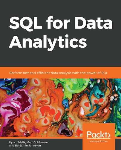
- Query plan the emails table and set the limit as 5. Enter the following statement into the PostgreSQL interpreter:
sqlda=# EXPLAIN SELECT * FROM emails LIMIT 5;
This repeats the previous statement, where the planner is limited to the first five records. This query will produce the following output from the planner:
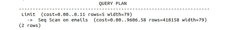
Figure 8.9: Query plan with limited rows
Referring to Figure 8.9, we can see that there are two individual rows in the plan. This indicates that the plan is composed of two separate steps, with the lower line of the plan (or, in this case, the first step to be executed) being a repeat of that shown in Figure 8.8. The upper line of the plan is the component that limits the result to only 5 rows. The Limit process is an additional cost of the query; however, it is quite insignificant compared to the lower-level plan, which retrieves approximately 418158 rows at a cost of 9606 pages requests. The Limit stage only returns 5 rows at a cost of 0.11 page requests.
Note
The overall estimated cost for a request comprises the time taken to retrieve the information from the disk as well as the number of rows that need to be scanned. The internal parameters, seq_page_cost and cpu_tuple_cost, define the cost of the corresponding operations within the tablespace for the database. While not recommended at this stage, these two variables can be changed to modify the steps prepared by the planner.
For more information, refer to the PostgreSQL documentation: https://www.postgresql.org/docs/current/runtime-config-query.html.
- Now, employ a more involved query, searching for dates between two specific values in the clicked_date column. Enter the following statement into the PostgreSQL interpreter:
sqlda=# EXPLAIN SELECT * FROM emails WHERE clicked_date BETWEEN '2011-01-01' and '2011-02-01';
This will produce the following query plan:

Figure 8.10: Sequential scan for searching dates between two specific values
The first aspect of this query plan to note is that it comprises a few different steps. The lower-level query is similar to the previous query in that it executes a sequential scan. However, rather than limiting the output, we are filtering it on the basis of the timestamp strings provided. Notice that the sequential scan is to be completed in parallel, as indicated by the Parallel Seq Scan, and the fact that two workers are planned to be used. Each individual sequence scan should return approximately 54 rows, taking a cost of 8038.49 to complete. The upper level of the plan is a Gather state, which is executed at the start of the query. We can see here for the first time that the upfront costs are non-zero (1,000) and total 9051.49, including the gather and search steps.
In this exercise, we worked with the query planner and the output of the EXPLAIN command. These relatively simple queries highlighted a number of the features of the SQL query planner as well as the detailed information that is provided by it. Having a good understanding of the query planner and the information it is returning to you will serve you well in your data science endeavors. Just remember that this understanding will come with time and practice; never hesitate to consult the PostgreSQL documentation: https://www.postgresql.org/docs/current/using-explain.html.
We will continue to practice reading query plans throughout this chapter as we look at different scan types and the methods, they use to improve performance.
Activity 10: Query Planning
Our aim in this activity is to query plan for reading and interpreting the information returned by the planner. Let's say that we are still dealing with our sqlda database of customer records and that our finance team would like us to implement a system to regularly generate a report of customer activity in a specific geographical region. To ensure that our report can be run in a timely manner, we need an estimate of how long the SQL queries will take. We will use the EXPLAIN command to find out how long some of the report queries will take:
- Open PostgreSQL and connect to the sqlda database.
- Use the EXPLAIN command to return the query plan for selecting all available records within the customers table.
- Read the output of the plan and determine the total query cost, the setup cost, the number of rows to be returned, and the width of each row. Looking at the output, what are the units for each of the values returned from the plan after performing this step?
- Repeat the query from step 2 of this activity, this time limiting the number of returned records to 15.
Looking at the updated query plan, how many steps are involved in the query plan? What is the cost of the limiting step?
- Generate the query plan, selecting all rows where customers live within a latitude of 30 and 40 degrees. What is the total plan cost as well as the number of rows returned by the query?
Expected output:
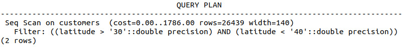
Figure 8.11: Plan for customers living within a latitude of 30 and 40 degrees
Note
The solution to the activity can be found on page 340. For an additional challenge, try completing this exercise in Python using psycopg2.
In this activity, we practiced reading the plans returned by the query planner. As discussed previously, plan reading requires substantial practice to master it. This activity began this process and it is strongly recommended that you frequently use the EXPLAIN command to improve your plan reading.
Index Scanning
Index scans are one method of improving the performance of our database queries. Index scans differ from sequential scan in that a pre-processing step is executed before the search of database records can occur. The simplest way to think of an index scan is just like the index of a text or reference book. In writing a non-fiction book, a publisher parses through the contents of the book and writes the page numbers corresponding with each alphabetically sorted topic. Just as the publisher goes to the initial effort of creating an index for the reader's reference, so we can create a similar index within the PostgreSQL database. This index within the database creates a prepared and organized set or a subset of references to the data under specified conditions. When a query is executed and an index is present that contains information relevant to the query, the planner may elect to use the data that was pre-processed and pre-arranged within the index. Without using an index, the database needs to repeatedly scan through all records, checking each record for the information of interest.
Even if all of the desired information is at the start of the database, without indexing, the search will still scan through all available records. Clearly, this would take a significantly longer time than necessary.
There are a number of different indexing strategies that PostgreSQL can use to create more efficient searches, including B-trees, hash indexes, Generalized Inverted Indexes (GINs), and Generalized Search Trees (GISTs). Each of these different index types has its own strengths and weaknesses and, hence, is used in different situations. One of the most frequently used indexes is the B-tree, which is the default indexing strategy used by PostgreSQL and is available in almost all database software. We will first spend some time investigating the B-tree index, looking at what makes it useful as well as some of its limitations.
The B-tree Index
The B-tree index is a type of binary search tree and is characterized by the fact that it is a self-balancing structure, maintaining its own data structure for efficient searching. A generic B-tree structure can be found in Figure 8.12, in which we can see that each node in the tree has no more than two elements (thus providing balance) and that the first node has two children. These traits are common among B-trees, where each node is limited to n components, thus forcing the split into child nodes. The branches of the trees terminate at leaf nodes, which, by definition, have no children:
Figure 8.12: Generic B-tree
Using Figure 8.12 as an example, say we were looking for the number 13 in the B-tree index. We would start at the first node and select whether the number was less than 5 or greater than 10. This would lead us down the right-hand branch of the tree, where we would again choose between less than 15 and greater than 20. We would then select less than 15 and arrive at the location of 13 in the index. We can see immediately that this operation would be much faster than looking through all available values. We can also see that for performance, the tree must be balanced to allow for an easy path for traversal. Additionally, there must be sufficient information to allow splitting. If we had a tree index with only a few possible values to split on and a large number of samples, we would simply divide the data into a few groups.
Considering B-trees in the context of database searching, we can see that we require a condition to divide the information (or split) on, and we also need sufficient information for a meaningful split. We do not need to worry about the logic of following the tree, as that will be managed by the database itself and can vary depending on the conditions for searching. Even so, it is important for us to understand the strengths and weaknesses of the method to allow us to make appropriate choices when creating the index for optimal performance.
To create an index for a set of data, we use the following syntax:
CREATE INDEX <index name> ON <table name>(table column);
We can also add additional conditions and constraints to make the index more selective:
CREATE INDEX <index name> ON <table name>(table column) WHERE [condition];
We can also specify the type of index:
CREATE INDEX <index name> ON <table name> USING TYPE(table column)
For example:
CREATE INDEX ix_customers ON customers USING BTREE(customer_id);
In the next exercise, we will start with a simple plan and work our way through more complicated queries and query plans using index scans.
Exercise 27: Creating an Index Scan
In this exercise, we will create a number of different index scans and will investigate the performance characteristics of each of the scans.
Continuing with the scenario from the previous activity, say we had completed our report service but wanted to make the queries faster. We will try to improve this performance using indexing and index scans. You will recall that we are using a table of customer information that includes contact details such as name, email address, phone number, and address information, as well as the latitude and longitude details of their address. The following are the steps to perform:
- Ensure that the sqlda database is loaded as described within the Preface. Retrieve the Exercise27.sql file from the accompanying source code. This file will contain all the queries used throughout this exercise; however, we will enter them manually using the SQL interpreter to reinforce our understanding of the query planner's operation.
Note
This file can be downloaded from the accompanying source code available at https://github.com/TrainingByPackt/SQL-for-Data-Analytics/blob/master/Lesson08/Exercise27.
- Open PostgreSQL and connect to the sqlda database:
C:> psql sqlda
Upon successful connection, you will be presented with the interface to the PostgreSQL database:

Figure 8.13: PostgreSQL interpreter
- Starting with the customers database, use the EXPLAIN command to determine the cost of the query and the number of rows returned in selecting all of the entries with a state value of FO:
sqlda=# EXPLAIN SELECT * FROM customers WHERE state='FO';
The following is the output of the preceding code:

Figure 8.14: Query plan of a sequential scan with constraint
Note that there is only 1 row returned and that the setup cost is 0, but the total query cost is 1661.
- Determine how many unique state values there are, again using the EXPLAIN command:
sqlda=# EXPLAIN SELECT DISTINCT state FROM customers;
The output is as follows:

Figure 8.15: Unique state values
So, there are 51 unique values within the state column.
- Create an index called ix_state using the state column of customers:
sqlda=# CREATE INDEX ix_state ON customers(state);
- Rerun the EXPLAIN statement from step 5:
sqlda=# EXPLAIN SELECT * FROM customers WHERE state='FO';
The following is the output of the preceding code:

Figure 8.16: Query plan of an index scan on the customers table
Notice that an index scan is now being used using the index we just created in step 5. We can also see that we have a non-zero setup cost (0.29), but the total cost is very much reduced, from the previous 1661 to only 8.31! This is the power of the index scan.
Now, let's look at a slightly different example, looking at the time it takes to return a search on the gender column.
- Use the EXPLAIN command to return the query plan for a search for all records of males within the database:
sqlda=# EXPLAIN SELECT * FROM customers WHERE gender='M';
The output is as follows:

Figure 8.17: Query plan of a sequential scan on the customers table
- Create an index called ix_gender using the gender column of customers:
sqlda=# CREATE INDEX ix_state ON customers(gender);
- Confirm the presence of the index using d:
d customers;
Scrolling to the bottom, we can see the indexes using the ix_ prefix, as well as the column from the table used to create the index:
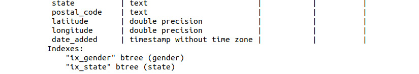
Figure 8.18: Structure of the customers table
- Rerun the EXPLAIN statement from step 10:
sqlda=# EXPLAIN SELECT * FROM customers WHERE gender='M';
The following is the output of the preceding code:

Figure 8.19: Query plan output of a sequential scan with a condition statement
Notice that the query plan has not changed at all, despite the use of the index scan. This is because there is insufficient information to create a useful tree within the gender column. There are only two possible values, M and F. The gender index essentially splits the information in two; one branch for males, and one for females. The index has not split the data into branches of the tree well enough to gain any benefit. The planner still needs to sequentially scan through at least half of the data, and so it is not worth the overhead of the index. It is for this reason that the query planner insists on not using the index.
- Use EXPLAIN to return the query plan, searching for latitudes less than 38 degrees and greater than 30 degrees:
sqlda=# EXPLAIN SELECT * FROM customers WHERE (latitude < 38) AND (latitude > 30);
The following is the output of the preceding code:
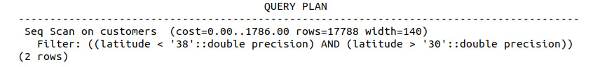
Figure 8.20: Query plan of a sequential scan on the customers table with a multi-factor conditional statement
Notice that the query is using a sequential scan with a filter. The initial sequential scan returns 17788 before the filter and costs 1786 with 0 start up cost.
- Create an index called ix_latitude using the latitude column of customers:
sqlda=# CREATE INDEX ix_latitude ON customers(latitude);
- Rerun the query of step 11 and observe the output of the plan:
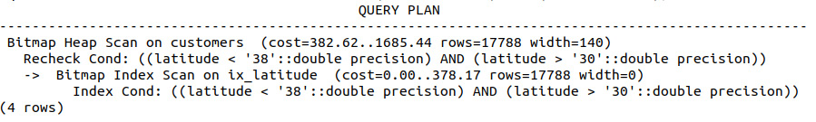
Figure 8.21: Observe the plan after rerunning the query
We can see that the plan is a lot more involved than the previous one, with a bitmap heap scan and a bitmap index scan being used. We will cover bitmap scans soon, but first, let's get some more information by adding the ANALYZE command to EXPLAIN.
- Use EXPLAIN ANALYZE to query plan the content of the customers table with latitude values of between 30 and 38:
sqlda=# EXPLAIN ANALYZE SELECT * FROM customers WHERE (latitude < 38) AND (latitude > 30);
The following output will be displayed:
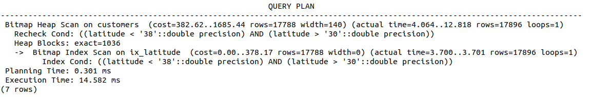
Figure 8.22: Query plan output containing additional EXPLAIN ANALYZE content
With this extra information, we can see that there is 0.3 ms of planning time and 14.582 ms of execution time, with the index scan taking almost the same amount of time to execute as the bitmap heat scan takes to start.
- Now, let's create another index where latitude is between 30 and 38 on the customers table:
sqlda=# CREATE INDEX ix_latitude_less ON customers(latitude) WHERE (latitude < 38) and (latitude > 30);
- Re-execute the query of step 15 and compare the query plans:
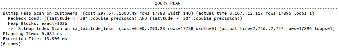
Figure 8.23: Query plan displaying the trade-off between planning and execution time
Using this more targeted index, we were able to shave 0.681 ms off the execution time, at the cost of an additional 0.3 ms of planning time.
Thus, we have squeezed some additional performance out of our query as our indexes have made the searching process more efficient. We may have had to pay an upfront cost to create the index, but once created, repeat queries can be executed more quickly.
Activity 11: Implementing Index Scans
In this activity, we will determine whether index scans can be used to reduce query time. After creating our customer reporting system for the marketing department in Activity 10: Query Planning, we have received another request to allow records to be identified by their IP address or the associated customer names. We know that there are a lot of different IP addresses and we need performant searches. Plan out the queries required to search for records by IP address as well as for certain customers with the suffix Jr in their name.
Here are the steps to follow:
- Use the EXPLAIN and ANALYZE commands to profile the query plan to search for all records with an IP address of 18.131.58.65. How long does the query take to plan and execute?
- Create a generic index based on the IP address column.
- Rerun the query of step 1. How long does the query take to plan and execute?
- Create a more detailed index based on the IP address column with the condition that the IP address is 18.131.58.65.
- Rerun the query of step 1. How long does the query take to plan and execute? What are the differences between each of these queries?
- Use the EXPLAIN and ANALYZE commands to profile the query plan to search for all records with a suffix of Jr. How long does the query take to plan and execute?
- Create a generic index based on the suffix address column.
- Rerun the query of step 6. How long does the query take to plan and execute?
Expected output
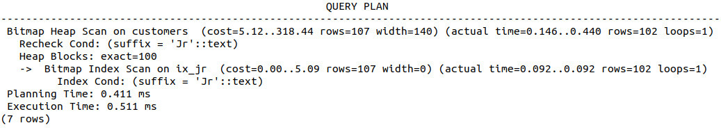
Figure 8.24: Query plan of the scan after creating an index on the suffix column
Note
The solution to the activity can be found on page 341.
In this activity, we have squeezed some additional performance out of our query as our indexes have made the searching process more efficient. We will learn how the hash index works in the next section.
Hash Index
The final indexing type we will cover is the hash index. The hash index has only recently gained stability as a feature within PostgreSQL, with previous versions issuing warnings that the feature is unsafe and reporting that the method is typically not as performant as B-tree indexes. At the time of writing, the hash index feature is relatively limited in the comparative statements it can run, with equality (=) being the only one available. So, given that the feature is only just stable and somewhat limited in options for use, why would anyone use it? Well, hash indices are able to describe large datasets (in the order of tens of thousands of rows or more) using very little data, allowing more of the data to be kept in memory and reducing search times for some queries. This is particularly important for databases that are at least several gigabytes in size.
A hash index is an indexing method that utilizes a hash function to achieve its performance benefits. A hash function is a mathematical function that takes data or a series of data and returns a unique length of alphanumeric characters depending upon what information was provided and the unique hash code used. Let's say we had a customer named "Josephine Marquez." We could pass this information to a hash function, which could produce a hash result such as 01f38e. Say we also had records for Josephine's husband, Julio; the corresponding hash for Julio could be 43eb38a. A hash map uses a key-value pair relationship to find data.
We could (but are not limited to) use the values of a hash function to provide the key, using the data contained in the corresponding row of the database as the value. As long as the key is unique to the value, we can quickly access the information we require. This method can also reduce the overall size of the index in memory, if only the corresponding hashes are stored, thereby dramatically reducing the search time for a query.
The following example shows how to create a hash index:
sqlda=# CREATE INDEX ix_gender ON customers USING HASH(gender);
You will recall that the query planner is able to ignore the indices created if it deems them to be not significantly faster for the existing query or just not appropriate. As the hash scan is somewhat limited in use, it may not be uncommon for a different search to ignore the indices.
Exercise 28: Generating Several Hash Indexes to Investigate Performance
In this exercise, we will generate a number of hash indexes and investigate the potential performance increases that can be gained from using them. We will start the exercise by rerunning some of the queries of previous exercises and comparing the execution times:
- Drop all existing indexes using the DROP INDEX command:
DROP INDEX <index name>;
- Use EXPLAIN and ANALYZE on the customer table where the gender is male, but without using a hash index:
sqlda=# EXPLAIN ANALYZE SELECT * FROM customers WHERE gender='M';
The following output will be displayed:
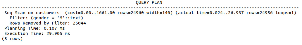
Figure 8.25: Standard sequential scan
We can see here that the estimated planning time is 0.107 ms and the execution time is 29.905 ms.
- Create a B-tree index on the gender column and repeat the query to determine the performance using the default index:
sqlda=# CREATE INDEX ix_gender ON customers USING btree(gender);
sqlda=#
The following is the output of the preceding code:
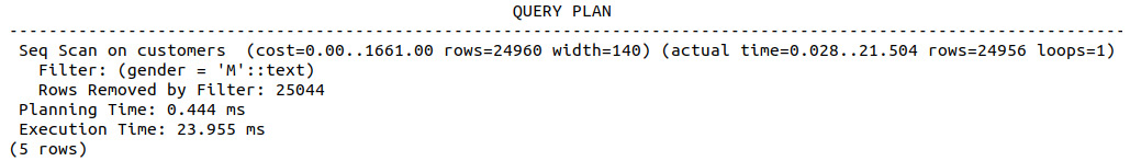
Figure 8.26: Query planner ignoring the B-tree index
We can see here that the query planner has not selected the B-tree index, but rather the sequential scan. The costs of the scans do not differ, but the planning and execution time estimates have been modified. This is not unexpected, as these measures are exactly that – estimates based on a variety of different conditions, such as data in memory and I/O constraints.
- Repeat the following query at least five times manually and observe the time estimates after each execution:
sqlda=# EXPLAIN ANALYZE SELECT * FROM customers WHERE gender='M';
The results of the five individual queries can be seen in the following screenshot; note that the planning and execution times differ for each separate execution of the query:
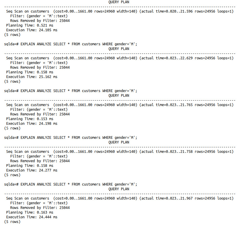
Figure 8.27: Five repetitions of the same sequential scan
- Drop or remove the index:
sqlda=# DROP INDEX ix_gender;
- Create a hash index on the gender column:
sqlda=# CREATE INDEX ix_gender ON customers USING HASH(gender);
- Repeat the query from step 4 to see the execution time:
sqlda=# EXPLAIN ANALYZE SELECT * FROM customers WHERE gender='M';
The following output will be displayed:
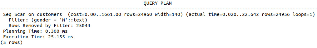
Figure 8.28: Query planner ignoring the hash index
As with the B-tree index, there was no benefit to using the hash index on the gender column, and so it was not used by the planner.
- Use the EXPLAIN ANALYZE command to profile the performance of the query that selects all customers where the state is FO:
sqlda=# EXPLAIN ANALYZE SELECT * FROM customers WHERE state='FO';
The following output will be displayed:
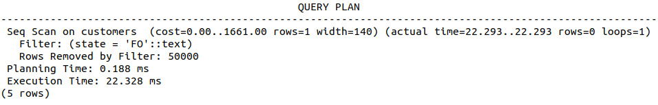
Figure 8.29: Sequential scan with filter by specific state
- Create a B-tree index on the state column of the customers table and repeat the query profiling:
sqlda=# CREATE INDEX ix_state ON customers USING BTREE(state);
sqlda=# EXPLAIN ANALYZE SELECT * FROM customers WHERE state='FO';
The following is the output of the preceding code:
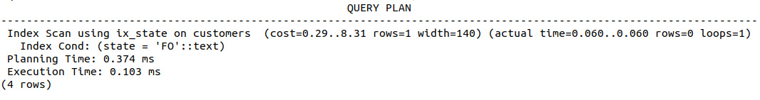
Figure 8.30: Performance benefit due to B-tree indexing
Here, we can see a significant performance increase due to the B-tree index with a slight setup cost. How does the hash scan perform? Given that the execution time has dropped from 22.3 ms to 0.103 ms, it is reasonable to conclude that the increased planning cost has increased by approximately 50%.
- Drop the ix_state B-tree index and create a hash scan:
sqlda=# DROP INDEX ix_state;
sqlda=# CREATE INDEX ix_state ON customers USING HASH(state);
- Use EXPLAIN and ANALYZE to profile the performance of the hash scan:
sqlda=# EXPLAIN ANALYZE SELECT * FROM customers WHERE state='FO';
The following is the output of the preceding code:
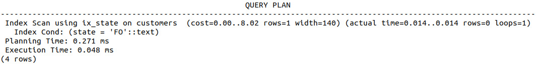
Figure 8.31: Additional performance boost using a hash index
We can see that, for this specific query, a hash index is particularly effective, reducing both the planning/setup time and cost of the B-tree index, as well as reducing the execution time to less than 1 ms from approximately 25 ms.
In this exercise, we used hash indexes to find the effectiveness of a particular query. We saw how the execution time goes down when using a hash index in a query.
Activity 12: Implementing Hash Indexes
In this activity, we will investigate the use of hash indexes to improve performance using the emails table from the sqlda database. We have received another request from the marketing department. This time, they would like us to analyze the performance of an email marketing campaign. Given that the success rate of email campaigns is low, many different emails are sent to many customers at a time. Use the EXPLAIN and ANALYZE commands to determine the planning time and cost, as well as the execution time and cost, of selecting all rows where the email subject is Shocking Holiday Savings On Electric Scooters:
- Use the EXPLAIN and ANALYZE commands to determine the planning time and cost, as well as the execution time and cost, of selecting all rows where the email subject is Shocking Holiday Savings On Electric Scooters in the first query and Black Friday. Green Cars. in the second query.
- Create a hash scan on the email_subject column.
- Repeat step 1. Compare the output of the query planner without the hash index to that with the hash index. What effect did the hash scan have on the performance of the two queries?
- Create a hash scan on the customer_id column.
- Use EXPLAIN and ANALYZE to estimate how long it would take to select all rows with a customer_id value greater than 100. What type of scan was used and why?
Expected output:
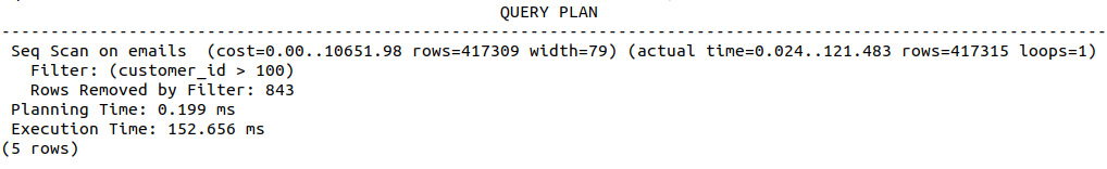
Figure 8.32: Query planner ignoring the hash index due to limitations
Note
The solution to the activity can be found on page 343.
In this activity, a sequential scan was used in this query rather than the hash scan created due to the current limitations of hash scan usage. At the time of writing, use of the hash scan is limited to equality comparisons, which involves searching for values equal to a given value.
Effective Index Use
So far in this chapter, we have looked at a number of different scanning methods, and the use of both B-trees and hash scans as a means of reducing query times. We have also presented a number of different examples of where an index was created for a field or condition and was explicitly not selected by the query planner when executing the query as it was deemed a more inefficient choice. In this section, we will spend some time discussing the appropriate use of indexes for reducing query times, since, while indexes may seem like an obvious choice for increasing query performance, this is not always the case. Consider the following situations:
- The field you have used for your index is frequently changing: In this situation, where you are frequently inserting or deleting rows in a table, the index that you have created may quickly become inefficient as it was constructed for data that is either no longer relevant or has since had a change in value. Consider the index at the back of this book. If you move the order of the chapters around, the index is no longer valid and would need to be republished. In such a situation, you may need to periodically re-index the data to ensure the references to the data are up to date. In SQL, we can rebuild the data indices by using the REINDEX command, which leads to a scenario where you will need to consider the cost, means, and strategy of frequent re-indexing versus other performance considerations, such as the query benefits introduced by the index, the size of the database, or even whether changes to the database structure could avoid the problem altogether.
- The index is out of date and the existing references are either invalid or there are segments of data without an index, preventing use of the index by the query planner: In such a situation, the index is so old that it cannot be used and thus needs to be updated.
- You are frequently looking for records containing the same search criteria within a specific field: We considered an example similar to this when looking for customers within a database whose records contained latitude values of less than 38 and greater than 30, using SELECT * FROM customers WHERE (latitude < 38) and (latitude > 30). In this example, it may be more efficient to create a partial index using the subset of data, as here: CREATE INDEX ix_latitude_less ON customers(latitude) WHERE (latitude < 38) and (latitude > 30). In this way, the index is only created using the data we are interested in, and is thereby smaller in size, quicker to scan, easier to maintain, and can also be used in more complex queries.
- The database isn't particularly large: In such a situation, the overhead of creating and using the index may simply not be worth it. Sequential scans, particularly those using data already in RAM, are quite fast, and if you create an index on a small dataset, there is no guarantee that the query planner will use it or get any significant benefit from using it.
Performant Joins
The JOIN functionality in SQL-compliant databases provides a very powerful and efficient method of combining data from different sources, without the need for complicated looping structures or a series of individual SQL statements. We covered joins and join theory in detail in Chapter 3, SQL for Data Preparation. As suggested by the name of the command, a join takes information from two or more tables and uses the contents of the records within each table to combine the two sets of information. Because we are combining this information without the use of looping structures, this can be done very efficiently. In this section, we will consider the use of joins as a more performant alternative to looping structures. The following is the Customer Information table:

Figure 8.33: Customer information
The following table shows the Order Information table:

Figure 8.34: Order information
So, with this information, we may want to see whether there are some trends in the items that are sold based on the customer's address. We can use JOIN to bring these two sets of information together; we will use the Customer ID column to combine the two datasets and produce the information shown in the following table:
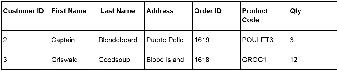
Figure 8.35: Join by customer ID
We can see in the preceding example that the join included all of the records where there was information available for both the customer and the order. As such, the customer Meat Hook was omitted from the combined information since no order information was available. In the example, we executed INNER JOIN; there are, however, a number of different joins available, and we will spend some time looking through each of them. The following is an example that shows the use of a performant INNER JOIN:
smalljoins=# EXPLAIN ANALYZE SELECT customers.*, order_info.order_id, order_info.product_code, order_info.qty FROM customers INNER JOIN order_info ON customers.customer_id=order_info.customer_id;
Refer to Chapter 3, SQL for Data Preparation, for more information on joins. In the next exercise, we will investigate the use of performant inner joins.
Exercise 29: Determining the Use of Inner Joins
In this exercise, we will investigate the use of inner joins to efficiently select multiple rows of data from two different tables. Let's say that our good friends in the marketing department gave us two separate databases: one from SalesForce and one from Oracle. We could use a JOIN statement to merge the corresponding information from the two sources into a single source. Here are the steps to follow:
- Create a database called smalljoins on the PostgreSQL server:
$ createdb smalljoins
- Load the smalljoins.dump file provided in the accompanying source code from the GitHub repository: https://github.com/TrainingByPackt/SQL-for-Data-Analytics/blob/master/Datasets/smalljoins.dump:
$psql smalljoins < smalljoins.dump
- Open the database:
$ psql smalljoins
- Inspect the information available for customers:
smalljoins=# SELECT * FROM customers;
The following figure shows the output of the preceding code:
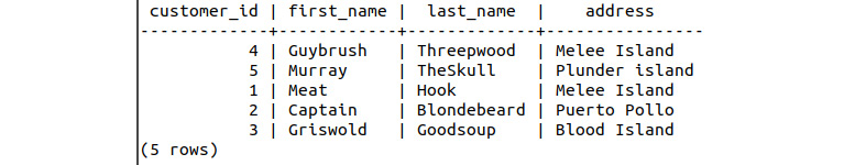
Figure 8.36: Customer table
- Inspect the information available for the order information:
smalljoins=# SELECT * FROM order_info;
This will display the following output:

Figure 8.37: Order information table
- Execute an inner join where we retrieve all columns from both tables without duplicating the customer_id column to replicate the results from Figure 8.35. We will set the left table to be customers and the right table to be order_info. So, to be clear, we want all columns from customers and the order_id, product_code, and qty columns from order_info when a customer has placed an order. Write this as a SQL statement:
smalljoins=# SELECT customers.*, order_info.order_id, order_info.product_code, order_info.qty FROM customers INNER JOIN order_info ON customers.customer_id=order_info.customer_id;
The following figure shows the output of the preceding code:
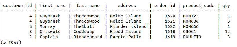
Figure 8.38 Join of customer and order information
- Save the results of this query as a separate table by inserting the INTO table_name keywords:
smalljoins=# SELECT customers.*, order_info.order_id, order_info.product_code, order_info.qty INTO join_results FROM customers INNER JOIN order_info ON customers.customer_id=order_info.customer_id;
The following figure shows the output of the preceding code:

Figure 8.39: Save results of join to a new table
- Use EXPLAIN ANALYZE to get an estimate of the time taken to execute the join. Now, how much faster is the join?
smalljoins=# EXPLAIN ANALYZE SELECT customers.*, order_info.order_id, order_info.product_code, order_info.qty FROM customers INNER JOIN order_info ON customers.customer_id=order_info.customer_id;
This will display the following output:
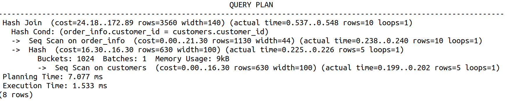
Figure 8.40: Baseline reading for comparing the performance of JOIN
- Select all of the customer_id values that are in order_info and use EXPLAIN ANALYZE to find out how long it takes to execute these individual queries:
smalljoins=# EXPLAIN ANALYZE SELECT * FROM customers WHERE customer_id IN (SELECT customer_id FROM order_info);
The following screenshot shows the output of the preceding code:
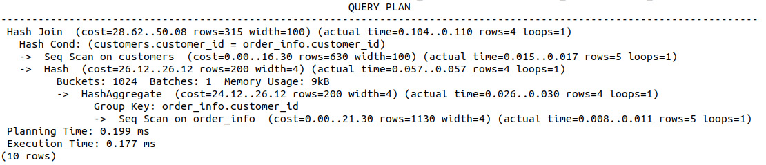
Figure 8.41: Improved performance of JOIN using a hash index
Looking at the results of the two query planners, we can see that not only did the inner join take about a third of the time of the sequential query (0.177 ms compared with 1.533 ms), but also that we have returned more information by the inner join, with order_id, product_code, and qty also being returned.
- Execute a left join using the customers table as the left table and order_info as the right table:
smalljoins=# SELECT customers.*, order_info.order_id, order_info.product_code, order_info.qty FROM customers LEFT JOIN order_info ON customers.customer_id=order_info.customer_id;
The following screenshot shows the output of the preceding code:
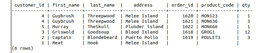
Figure 8.42: Left join of the customers and order_info tables
Notice the differences between the left join and the inner join. The left join has included the result for customer_id 4 twice, and has included the result for Meat Hook once, although there is no order information available. It has included the results of the left table with blank entries for information that is not present in the right table.
- Use EXPLAIN ANALYZE to determine the time and cost of executing the join:
smalljoins=# EXPLAIN ANALYZE SELECT customers.*, order_info.order_id, order_info.product_code, order_info.qty FROM customers LEFT JOIN order_info ON customers.customer_id=order_info.customer_id;
This will display the following output:
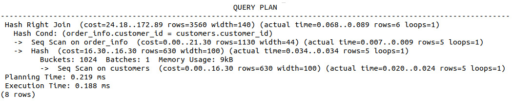
Figure 8.43: Query planner for executing the left join
- Replace the left join of step 11 with a right join and observe the results:
smalljoins=# EXPLAIN ANALYZE SELECT customers.*, order_info.order_id, order_info.product_code, order_info.qty FROM customers RIGHT JOIN order_info ON customers.customer_id=order_info.customer_id;
The following screenshot shows the output of the preceding code:
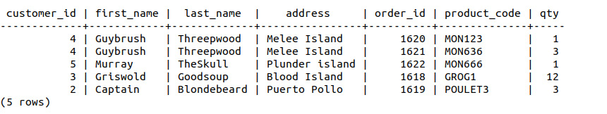
Figure 8.44: Results of a right join
Again, we have two entries for customer_id 4, Guybrush Threepwood, but we can see that the entry for customer_id 1, Meat Hook, is no longer present as we have joined on the basis of the information within the contents of the order_id table.
- Use EXPLAIN ANALYZE to determine the time and cost of the right join:
smalljoins=# EXPLAIN ANALYZE SELECT customers.*, order_info.order_id, order_info.product_code, order_info.qty FROM customers RIGHT JOIN order_info ON customers.customer_id=order_info.customer_id;
The following screenshot shows the output of the preceding code:
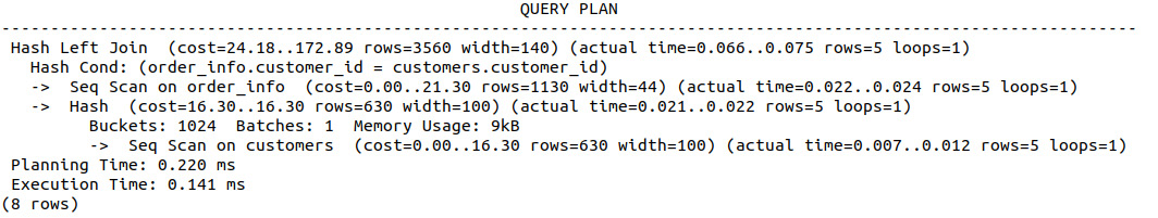
Figure 8.45: Query plan of a right join
We can see that the right join was marginally faster and more cost effective, which can be attributed to one less row being returned than in the left join.
- Insert an additional row into order_info with a customer_id value that is not present in the customers table:
smalljoins=# INSERT INTO order_info (order_id, customer_id, product_code, qty) VALUES (1621, 6, 'MEL386', 1);
- Replace the left join of step 11 with a full outer join and observe the results:
smalljoins=# SELECT customers.*, order_info.order_id, order_info.product_code, order_info.qty FROM customers FULL OUTER JOIN order_info ON customers.customer_id=order_info.customer_id;
This will display the following output:
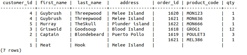
Figure 8.46: Results of a full outer join
Notice the line that contains product_code MEL386, but no information regarding the customer; there's a similar case for the line for customer_id Meat Hook. The full outer join has combined all available information even if some of the information is not available from either table.
- Use the EXPLAIN ANALYZE command to determine the performance of the query.
smalljoins=# EXPLAIN ANALYZE SELECT customers.*, order_info.order_id, order_info.product_code, order_info.qty FROM customers FULL OUTER JOIN order_info ON customers.customer_id=order_info.customer_id;
The following screenshot shows the output of the preceding code:
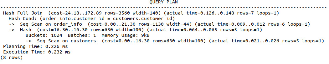
Figure 8.47: Query plan of a full outer join
The performance is very similar to that of the other queries, given that an additional row is provided, which can be clearly seen in the final output.
In this exercise, we were introduced to the usage and performance benefits of joins. We observed the combination of information from two separate tables using fewer resources than individual searches require, as well as the use of OUTER JOIN to efficiently combine all information. In the next activity, we will build upon our understanding of joins with a much larger dataset.
Activity 13: Implementing Joins
In this activity, our goal is to implement various performant joins. In this activity, we will use joins to combine information from a table of customers as well as information from a marketing email dataset. Say we have just collated a number of different email records from a variety of different databases. We would like to distill the information down into a single table so that we can perform some more detailed analysis. Here are the steps to follow:
- Open PostgreSQL and connect to the sqlda database.
- Determine a list of customers (customer_id, first_name, and last_name) who had been sent an email, including information for the subject of the email and whether they opened and clicked on the email. The resulting table should include the customer_id, first_name, last_name, email_subject, opened, and clicked columns.
- Save the resulting table to a new table, customer_emails.
- Find those customers who opened or clicked on an email.
- Find the customers who have a dealership in their city; customers who do not have a dealership in their city should have a blank value for the city columns.
- List those customers who do not have dealerships in their city (hint: a blank field is NULL).
Expected output
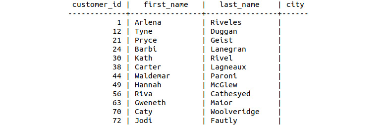
Figure 8.48: Customers without city information
The output shows the final list of customers in the cities where we have no dealerships.
Note
The solution to the activity can be found on page 346.
In this activity, we used joins to combine information from a table of customers as well as information from a marketing email dataset and helped the marketing manager to solve their query.
Functions and Triggers
So far in this chapter, we have discovered how to quantify query performance via the query planner, as well as the benefits of using joins to collate and extract information from multiple database tables. In this section, we will construct reusable queries and statements via functions, as well as automatic function execution via trigger callbacks. The combination of these two SQL features can be used to not only run queries or re-index tables as data is added to/updated in/removed from the database, but also to run hypothesis tests and track the results of the tests throughout the life of the database.
Function Definitions
As in almost all other programming or scripting languages, functions in SQL are contained sections of code, which provides a lot of benefits, such as efficient code reuse and simplified troubleshooting processes. We can use functions to repeat/modify statements or queries without re-entering the statement each time or searching for its use throughout longer code segments. One of the most powerful aspects of functions is also that they allow us to break the code into smaller, testable chunks. As the popular computer science expression goes "If the code is not tested, it cannot be trusted."
So, how do we define functions in SQL? There is a relatively straightforward syntax, with the SQL syntax keywords:
CREATE FUNCTION some_function_name (function_arguments)
RETURNS return_type AS $return_name$
DECLARE return_name return_type;
BEGIN
<function statements>;
RETURN <some_value>;
END; $return_name$
LANGUAGE PLPGSQL;
The following is a small explanation of the function used in the preceding code:
- some_function_name is the name issued to the function and is used to call the function at later stages.
- function_arguments is an optional list of function arguments. This could be empty, without any arguments provided, if we don't need any additional information to be provided to the function. To provide additional information, we can either use a list of different data types as the arguments (such as integer and numeric), or a list of arguments with parameter names (such as min_val integer and max_val numeric).
- return_type is the data type being returned from the function.
- return_name is the name of the variable to be returned (optional).
The DECLARE return_name return_type statement is only required if return_name is provided, and a variable is to be returned from the function. If return_name is not required, this line can be omitted from the function definition.
- function statements entail the SQL statements to be executed within the function.
- some_value is the data to be returned from the function.
- PLPGSQL specifies the language to be used in the function. PostgreSQL gives the ability to use other languages; however, their use in this context lies beyond the scope of this book.
Note
The complete PostgreSQL documentation for functions can be found at https://www.postgresql.org/docs/current/extend.html.
Exercise 30: Creating Functions without Arguments
In this exercise, we will create the most basic function – one that simply returns a constant value – so we can build up a familiarity with the syntax. We will construct our first SQL function that does not take any arguments as additional information. This function may be used to repeat SQL query statements that provide basic statistics about the data within the tables of the sqlda database. These are the steps to follow:
- Connect to the sqlda database:
$ psql sqlda
- Create a function called fixed_val that does not accept any arguments and returns an integer. This is a multi-line process. Enter the following line first:
sqlda=# CREATE FUNCTION fixed_val() RETURNS integer AS $$
This line starts the function declaration for fixed_val, and we can see that there are no arguments to the function, as indicated by the open/closed brackets, (), nor any returned variables.
- In the next line, notice that the characters within the command prompt have adjusted to indicate that it is awaiting input for the next line of the function:
sqlda$#
- Enter the BEGIN keyword (notice that as we are not returning a variable, the line containing the DECLARE statement has been omitted):
sqlda$# BEGIN
- We want to return the value 1 from this function, so enter the statement RETURN 1:
sqlda$# RETURN 1;
- End the function definition:
sqlda$# END; $$
- Finally, add the LANGUAGE statement, as shown in the following function definition:
sqlda-# LANGUAGE PLPGSQL;
This will complete the function definition.
- Now that the function is defined, we can use it. As with almost all other SQL statements we have completed to date, we simply use a SELECT command:
sqlda=# SELECT * FROM fixed_val();
This will display the following output:

Figure 8.49: Output of the function call
Notice that the function is called using the open and closed brackets in the SELECT statement.
- Use EXPLAIN and ANALYZE in combination with this statement to characterize the performance of the function:
sqlda=# EXPLAIN ANALYZE SELECT * FROM fixed_val();
The following screenshot shows the output of the preceding code:
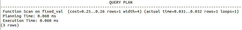
Figure 8.50: Performance of the function call
So far, we have seen how to create a simple function, but simply returning a fixed value is not particularly useful. We will now create a function that determines the number of samples in the sales table. Notice that the three rows being referenced in the preceding screesnhot refer not to the result of SELECT * FROM fixed_val(); but rather the result of the query planner. Looking at the first line of the information returned by the query planner, we can see that only one row of information is returned from the SELECT statement.
- Create a function called num_samples that does not take any arguments but returns an integer called total that represents the number of samples in the sales table:
sqlda=# CREATE FUNCTION num_samples() RETURNS integer AS $total$
- We want to return a variable called total, and thus we need to declare it. Declare the total variable as an integer:
sqlda$# DECLARE total integer;
- Enter the BEGIN keyword:
sqlda$# BEGIN
- Enter the statement that determines the number of samples in the table and assigns the result to the total variable:
sqlda$# SELECT COUNT(*) INTO total FROM sales;
- Return the value for total:
sqlda$# RETURN total;
- End the function with the variable name:
sqlda$# END; $total$
- Add the LANGUAGE statement as shown in the following function definition:
sqlda-# LANGUAGE PLPGSQL;
This will complete the function definition, and upon successful creation, the CREATE_FUNCTION statement will be shown.
- Use the function to determine how many rows or samples there are in the sales table:
sqlda=# SELECT num_samples();
The following figure shows the output of the preceding code:

Figure 8.51: Output of the num_samples function call
We can see that by using the SELECT statement in combination with our SQL function, there are 37,711 records within the sales database.
In this exercise, we have created our first user-defined SQL function and discovered how to create and return information from variables within the function.
Activity 14: Defining a Maximum Sale Function
Our aim here is to create a user-defined function so we can calculate the largest sale amount in a single function call. In this activity, we will reinforce our knowledge of functions as we create a function that determines the highest sale amount in a database. At this stage, our marketing department is starting to make a lot of data analysis requests and we need to be more efficient in fulfilling them, as they are currently just taking too long. Perform the following steps:
- Connect to the sqlda database.
- Create a function called max_sale that does not take any input arguments but returns a numeric value called big_sale.
- Declare the big_sale variable and begin the function.
- Insert the maximum sale amount into the big_sale variable.
- Return the value for big_sale.
- End the function with the LANGUAGE statement.
- Call the function to find what the biggest sale amount in the database is?
Expected output

Figure 8.52: Output of the maximum sales function call
Note
The solution to the activity can be found on page 348.
In this activity, we created a user-defined function to calculate the largest sale amount from a single function call using the MAX function.
Exercise 31: Creating Functions with Arguments Using a Single Function
Our goal is now to create a function that will allow us to calculate information from multiple tables using a single function. In this exercise, we will create a function that determines the average value from the sales amount column, with respect to the value of the corresponding channel. After creating our previous user-defined function to determine the biggest sale in the database, we have observed a significant increase in the efficiency with which we fulfill our marketing department's requests.
Perform the following steps to complete the exercise:
- Connect to the sqlda database:
$ psql sqlda
- Create a function called avg_sales that takes a text argument input, channel_type, and returns a numeric output:
sqlda=# CREATE FUNCTION avg_sales(channel_type TEXT) RETURNS numeric AS $channel_avg$
- Declare the numeric channel_avg variable and begin the function:
sqlda$# DECLARE channel_avg numeric;
sqlda$# BEGIN
- Determine the average sales_amount only when the channel value is equal to channel_type:
sqlda$# SELECT AVG(sales_amount) INTO channel_avg FROM sales WHERE channel=channel_type;
- Return channel_avg:
sqlda$# RETURN channel_avg;
- End the function and specify the LANGUAGE statement:
sqlda$# END; $channel_avg$
sqlda-# LANGUAGE PLPGSQL;
- Determine the average sales amount for the internet channel:
sqlda=# SELECT avg_sales('internet');
The following figure shows the output of the preceding code:

Figure 8.53: Output of the average sales function call with the internet parameter
Now do the same for the dealership channel:
sqlda=# SELECT avg_sales('dealership');
The following figure shows the output of the preceding code:

Figure 8.54: Output of the average sales function call with the dealership parameter
This output shows the average sales for a dealership, which is 7939.331.
In this exercise, we were introduced to using function arguments to further modify the behavior of functions and the outputs they return.
The df and sf commands
You can use the df command in PostgreSQL to get a list of functions available in memory, including the variables and data types passed as arguments:
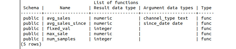
Figure 8.55: Result of the df command on the sqlda database
The sf function_name command in PostgreSQL can be used to review the function definition for already-defined functions:

Figure 8.56: Contents of the function using sf
Activity 15: Creating Functions with Arguments
In this activity, our goal is to create a function with arguments and compute the output. In this activity, we will construct a function that computes the average sales amount for transaction sales within a specific date range. Each date is to be provided to the function as a text string. These are the steps to follow:
- Create the function definition for a function called avg_sales_window that returns a numeric value and takes two DATE values to specify the from and to dates in the form YYYY-MM-DD.
- Declare the return variable as a numeric data type and begin the function.
- Select the average sales amount as the return variable where the sales transaction date is within the specified date.
- Return the function variable, end the function, and specify the LANGUAGE statement.
- Use the function to determine the average sales values between 2013-04-12 and 2014-04-12.
Expected output

Figure 8.57: Output of average sales since the function call
Note
The solution to the activity can be found on page 349.
In this activity, we constructed a function that computes the average sales amount for transaction sales within a specific date range from the database.
Triggers
Triggers, known as events or callbacks in other programming languages, are useful features that, as the name suggests, trigger the execution of SQL statements or functions in response to a specific event. Triggers can be initiated when one of the following happens:
- A row is inserted into a table
- A field within a row is updated
- A row within a table is deleted
- A table is truncated – that is, all rows are quickly removed from a table
The timing of the trigger can also be specified to occur:
- Before an insert, update, delete, or truncate operation
- After an insert, update, delete, or truncate operation
- Instead of an insert, update, delete, or truncate operation
Depending upon the context and the purpose of the database, triggers can have a wide variety of different use cases and applications. In a production environment where a database is being used to store business information and make process decisions (such as for a ride-sharing application or an e-commerce store), triggers can be used before any operation to create access logs to the database. These logs can then be used to determine who has accessed or modified the data within the database. Alternatively, triggers could be used to re-map database operations to a different database or table using the INSTEAD OF trigger.
In the context of a data analysis application, triggers can be used to either create datasets of specific features in real time (such as for determining the average of data over time or a sample-to-sample difference), test hypotheses concerning the data, or flag outliers being inserted/modified in a dataset.
Given that triggers are used frequently to execute SQL statements in response to events or actions, we can also see why functions are often written specifically for or paired with triggers. Self-contained, repeatable function blocks can be used for both trialing/debugging the logic within the function as well as inserting the actual code within the trigger. So, how do we create a trigger? Similarly, to the case with function definitions, there is a standard syntax; again, the SQL keywords:
CREATE TRIGGER some_trigger_name { BEFORE | AFTER | INSTEAD OF } { INSERT | DELETE | UPDATE | TRUNCATE } ON table_name
FOR EACH { ROW | STATEMENT }
EXECUTE PROCEDURE function_name ( function_arguments)
Looking at this generic trigger definition, we can see that there are a few individual components:
- We need to provide a name for the trigger in place of some_trigger_name.
- We need to select when the trigger is going to occur; either BEFORE, AFTER, or INSTEAD OF an event.
- We need to select what type of event we want to trigger on; either INSERT, DELETE, UPDATE, or TRUNCATE.
- We need to provide the table we want to monitor for events in table_name.
- The FOR EACH statement is used to specify how the trigger is to be fired. We can fire the trigger for each ROW that is within the scope of the trigger, or just once per STATEMENT despite the number of rows being inserted into the table.
- Finally, we just need to provide function_name and any relevant/required function_arguments to provide the functionality that we want to use on each trigger.
Some other functions that we will use are these:
- The get_stock function takes a product code as a TEXT input and returns the currently available stock for the specific product code.
- The insert_order function is used to add a new order to the order_info table and takes customer_id INTEGER, product_code TEXT, and qty INTEGER as inputs; it will return the order_id instance generated for the new record.
- The update_stock function will extract the information from the most recent order and will update the corresponding stock information from the products table for the corresponding product_code.
There are a number of different options available for SQL triggers that lie outside the scope of this book. For the complete trigger documentation, you can refer to https://www.postgresql.org/docs/current/sql-createtrigger.html.
Exercise 32: Creating Triggers to Update Fields
In this exercise, we will create a trigger that updates the fields whenever data is added. For this exercise, we will use the smalljoins database from the section of this chapter on joins and will create a trigger that updates the stock value within products for a product each time that an order is inserted into the order_info table. Using such a trigger, we can update our analysis in real time as end users interact with the database. These triggers will remove the need for us to run the analysis for the marketing department manually; instead, they will generate the results for us.
For this scenario, we will create a trigger to update the records for the available stock within the database for each of our products. As items are bought, the triggers will be fired, and the quantity of available stock will be updated. Here are the steps to perform:
- Load the prepared functions into the smalljoins database using the Functions.sql file which can be found in the accompanying source code, it is also available on GitHub: https://github.com/TrainingByPackt/SQL-for-Data-Analytics/tree/master/Lesson08/Exercise32.
$ psql smalljoins < Functions.sql
- Connect to the smalljoins database:
$ psql smalljoins
- Get a list of the functions using the df command after loading the function definitions:
smalljoins=# df
This will display the following output:
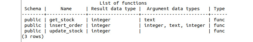
Figure 8.58: List of functions
- First, let's look at the current state of the products table:
smalljoins=# SELECT * FROM products;
The following figure shows the output of the preceding code:

Figure 8.59: List of products
For the order_info table, we can write the following query:
smalljoins=# SELECT * FROM order_info;
The following figure shows the output of the preceding code:

Figure 8.60: List of order information
- Insert a new order using the insert_order function with customer_id 4, product_code MON636, and qty 10:
smalljoins=# SELECT insert_order(4, 'MON636', 10);
The following figure shows the output of the preceding code:

Figure 8.61: Creating a new order
- Review the entries for the order_info table:
smalljoins=# SELECT * FROM order_info;
This will display the following output:

Figure 8.62: List of updated order information
Notice the additional row with order_id 1623.
- Update the products table to account for the newly sold 10 Red Herrings using the update_stock function:
smalljoins=# SELECT update_stock();
The following figure shows the output of the preceding code:

Figure 8.63: Call updated_stock function to update
This function call will determine how many Red Herrings are left in inventory (after the sales of the 10 additional herrings) and will update the table accordingly.
- Review the products table and notice the updated stock value for Red Herring:
smalljoins=# SELECT * FROM products;
The following figure shows the output of the preceding code:

Figure 8.64: List of updated product values
Updating the stock values manually will quickly become tedious. Let's create a trigger to do this automatically whenever a new order is placed.
- Delete (DROP) the previous update_stock function. Before we can create a trigger, we must first adjust the update_stock function to return a trigger, which has the benefit of allowing for some simplified code:
smalljoins=# DROP FUNCTION update_stock;
- Create a new update_stock function that returns a trigger. Note that the function definition is also contained within the Trigger.sql file for reference or direct loading into the database:
smalljoins=# CREATE FUNCTION update_stock() RETURNS TRIGGER AS $stock_trigger$
smalljoins$# DECLARE stock_qty integer;
smalljoins$# BEGIN
smalljoins$# stock_qty := get_stock(NEW.product_code) – NEW.qty;
smalljoins$# UPDATE products SET stock=stock_qty WHERE product_code=NEW.product_code;
smalljoins$# RETURN NEW;
smalljoins$# END; $stock_trigger$
smalljoins-# LANGUAGE PLPGSQL;
Note that in this function definition, we are using the NEW keyword followed by the dot operator (.) and the product_code (NEW.product_code) and qty (NEW.qty) field names from the order_info table. The NEW keyword refers to the record that was recently inserted, updated, or deleted and provides a reference to the information within the record.
In this exercise, we want the trigger to fire after the record is inserted into order_info and thus the NEW reference will contain this information. So, we can use the get_stock function with NEW.product_code to get the currently available stock for the record and simply subtract the NEW.qty value from the order record.
- Finally, let's create the trigger. We want the trigger to occur AFTER an INSERT operation on the order_info table. For each row, we want to execute the newly modified update_stock function to update the stock values in the product table:
smalljoins=# CREATE TRIGGER update_trigger
smalljoins-# AFTER INSERT ON order_info
smalljoins-# FOR EACH ROW
smalljoins-# EXECUTE PROCEDURE update_stock();
- Now that we have created a new trigger, let's test it. Call the insert_order function to insert a new record into the order_info table:
smalljoins=# SELECT insert_order(4, 'MON123', 2);
The following figure shows the output of the preceding code:

Figure 8.65: Insert a new order to use the trigger
- Look at the records from the order_info table:
smalljoins=# SELECT * FROM order_info;
This will display the following output:

Figure 8.66: Order information with an update from the trigger
- Look at the records for the products table:
smalljoins=# SELECT * FROM products;
The following figure shows the output of the preceding code:

Figure 8.67: Updated product information from the trigger
Our trigger worked! We can see that the available stock for the Rubber Chicken + Pulley MON123 has been reduced from 7 to 5, in accordance with the quantity of the inserted order.
In this exercise, we have successfully constructed a trigger to execute a secondary function following the insertion of a new record into the database.
Activity 16: Creating a Trigger to Track Average Purchases
Our goal here is to create a trigger for keeping track of the data that is updated. Let's say you are working as a data scientist for Monkey Islands, finest distributor of questionable and obscure items. The business is looking at trying a few different strategies to increase the number of items in each sale. To simplify your analysis, you decide to add a simple trigger that for each new order computes the average quantity in all the orders and puts the result in a new table along with the corresponding order_id. Here are the steps to follow:
- Connect to the smalljoins database.
- Create a new table called avg_qty_log that is composed of an order_id integer field and an avg_qty numeric field.
- Create a function called avg_qty that does not take any arguments but returns a trigger. The function computes the average value for all order quantities (order_info.qty) and inserts the average value, along with the most recent order_id, into avg_qty.
- Create a trigger called avg_trigger that calls the avg_qty function AFTER each row is inserted into the order_info table.
- Insert some new rows into the order_info table with quantities of 6, 7, and 8.
- Look at the entries in avg_qty_log. Is the average quantity of each order increasing?
Expected output

Figure 8.68: Average order quantity over time
Note
The solution to the activity can be found on page 350.
In this activity, we created a trigger for continuously keeping track of the data that is updated to analyze a product in the database.
Killing Queries
Sometimes, you have a lot of data, or perhaps insufficient hardware resources, and a query just runs for a very long time. In such a situation, you may need to stop the query, perhaps so you can implement an alternative query to get the information you need, but without the delayed response. In this section of the chapter, we are going to investigate how we can stop hanging, or, at least, hanging extremely long queries through the use of a secondary PostgreSQL interpreter. The following are some of the commands that we will use to kill queries:
- pg_sleep is a command that allows you to tell the SQL interpreter to essentially do nothing for the next period of time as defined by the input to the function in seconds.
- The pg_cancel_backend command causes the interpreter to end the query specified by the process ID (pid). The process will be terminated cleanly, allowing for appropriate resource cleanup. Clean termination should also be the first preference as it reduces the possibility of data corruption and damage to the database.
- The pg_terminate_background command stops an existing process but, as opposed to pg_cancel_background, forces the process to terminate without cleaning up any resources being used by the query. The query is immediately terminated, and data corruption may occur as a result.
Exercise 33: Canceling a Long Query
Our goal here is to learn how to cancel a long query to save time when we are stuck at query execution. You have been lucky enough to receive a large data store and you decided to run what you originally thought was a simple enough query to get some basic descriptive statistics of the data. For some reason, however, the query is taking an extremely long time and you are not even sure that it is running. You decide it is time to cancel the query, which means you would like to send a stop signal to the query but allow it sufficient time to clean up its resources gracefully. As there may be a wide variety of hardware available to us and the data required to induce a long query could be quite a lot to download, we will simulate a long query using the pg_sleep command. Here are the steps to follow.
For this exercise, you will require two separate SQL interpreter sessions running in separate windows, as shown in the following figure:
- Launch two separate interpreters by running psql sqlda:
C:> psql sqlda
This will display the following output in two separate windows:
Figure 8.69: Running multiple terminals
- In the first terminal, execute the sleep command with a parameter of 1000 seconds:
sqlda=# SELECT pg_sleep(1000);
After pressing Enter, you should notice that the cursor of the interpreter does not return:

Figure 8.70: Sleeping interpreter
- In the second terminal, select the pid and query columns from the pg_stat_activity table where state is active:
sqlda=# SELECT pid, query FROM pg_stat_activity WHERE state = 'active';
The following figure shows the output of the preceding code:
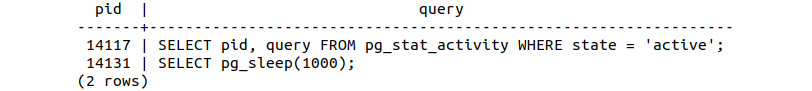
Figure 8.71: Active queries
- In the second terminal, pass the process ID of the pg_sleep query to the pg_cancel_backend command to terminate the pg_sleep query with a graceful cleanup:
sqlda=# SELECT pg_cancel_backend(14131);
The following figure shows the output of the preceding code:

Figure 8.72: Successful cancelation of the query
- Observe the first terminal and notice that the sleep command is no longer executing, as indicated by the return message:
Figure 8.73: Message indicating the cancelation of the query
This output screenshot shows an error as the query was canceled after the user's request.
In this exercise, we learned how to cancel a query that has taken a long time to execute.
Activity 17: Terminating a Long Query
Now our aim is to terminate a long query using the pg_terminate_background command just as we used pg_cancel_backend to stop the process. In this activity, we will consider the scenario as being one in which the cancelation of the query was not enough to stop the excessively long process. In such a situation, we require something a little heavier handed that, rather than requesting a clean termination of the process, forces a process to be terminated. Launch two separate SQL interpreters. Here are the steps to follow:
- In the first terminal, execute the sleep command with a parameter of 1000 seconds.
- In the second terminal, identify the process ID of the sleep query.
- Using the pid value, force the sleep command to terminate using the pg_terminate_background command.
- Verify in the first terminal that the sleep command has been terminated. Notice the message returned by the interpreter.
Expected output
Figure 8.74: Terminated pg_sleep process
Note
The solution to the activity can be found on page 352.
In this activity, we terminated a long-running query using the pg_terminate_background command.
Summary
In this chapter, we have covered a wide variety of topics all designed to help us understand and improve the performance of our SQL queries. The chapter began with a thorough discussion of the query planner, including the EXPLAIN and ANALYZE statements, as well as various indexing methods. We discussed a number of different compromises and considerations that can be made to reduce the time taken to execute queries. We considered a number of scenarios where indexing methods would be of benefit and others where the query planner may disregard the index, thus reducing the efficiency of the query. We then moved on to the use of joins to efficiently combine information from a number of different tables and ended with an in-depth look at functions and automatic function calls through the use of triggers.
In the next chapter, we will combine all of the topics we have covered thus far in a final case study, applying our SQL knowledge and the scientific method in general, as we solve a real-world problem.