Chapter 6

Importing and Exporting Data

Learning Objectives

By the end of this chapter, you will be able to:

• Use psql at the command line to efficiently interact with your database
• Use the COPY command to upload data to your database in bulk
• Use Excel to process data from your database
• Simplify your code using SQLAlchemy in Python
• Upload and download data to and from your database in bulk with R and Python

This chapter covers how to move data between your database and other analytics processing pipelines.

Introduction

In order to extract insights from your database, you need data. And, while it's possible that some of that data will be populated and updated for you, there are always going to be scenarios where you need more data that is not yet in your database. In this chapter, we are going to explore how we can efficiently upload data to our centralized database for further analysis.

Not only will we want to upload data to our database for further analysis, but there are also going to be times where we want to download data from our database for further processing. We will also explore the process of extracting data from our database.

One of the primary reasons you would want to upload or download data to or from your database is because you have other analytics tools that you want to use. You will often want to use other software to analyze your data. In this chapter, we will also look at how you can integrate your workflows with two specific programming languages that are frequently used for analytics: Python and R. These languages are powerful because they are easy to use, allow for advanced functionality, are open source, and have large communities supporting them as a result of their popularity. We will look at how large datasets can be passed between our programming languages and our databases efficiently so that we can have workflows that take advantage of all of the tools available to us.

With this in mind, we will start by looking at the bulk uploading and downloading functionality in the Postgres command-line client, psql, and then move on to importing and exporting data using Python and R.

The COPY Command

At this point, you are probably pretty familiar with the SELECT statement (covered in Chapter 2, The Basics of SQL for Analytics), which allows us to retrieve data from our database. While this command is useful for small datasets that can be scanned quickly, we will often want to save a large dataset to a file. By saving these datasets to files, we can further process or analyze the data locally using Excel, Python, or R. In order to retrieve these large datasets, we can use the Postgres COPY command, which efficiently transfers data from a database to a file, or from a file to a database.

Getting Started with COPY

The COPY statement retrieves data from your database and dumps it in the file format of your choosing. For example, take the following statement:

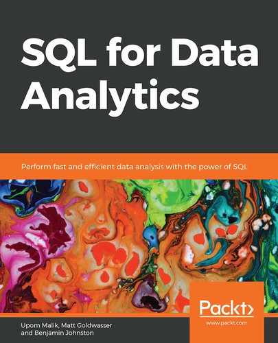
COPY (SELECT * FROM customers LIMIT 5) TO STDOUT WITH CSV HEADER;

Figure 6.1: Using COPY to print results to STDOUT in a CSV file format

This statement returns five rows from the table, with each record on a new line, and each value separated by a comma, in a typical .csv file format. The header is also included at the top.

Here is the breakdown of this command and the parameters that were passed in:

• COPY is simply the command used to transfer data to a file format.
• (SELECT * FROM customers LIMIT 5) is the query that we want to copy.
• TO STDOUT indicates that the results should be printed rather than saved to a file on the hard drive. "Standard Out" is the common term for displaying output in a command-line terminal environment.
• WITH is an optional keyword used to separate the parameters that we will use in the database-to-file transfer.
• CSV indicates that we will use the CSV file format. We could have also specified BINARY or left this out altogether and received the output in text format.
• HEADER indicates that we want the header printed as well.

  Note

  You can learn more about the parameters available for the COPY command in the Postgres documentation: https://www.postgresql.org/docs/current/sql-copy.html.

While the STDOUT option is useful, often, we will want to save data to a file. The COPY command offers functionality to do this, but data is saved locally on the Postgres server. You must specify the full file path (relative file paths are not permitted). If you have your Postgres database running on your computer, you can test this out using the following command:

COPY (SELECT * FROM customers LIMIT 5) TO '/path/to/my_file.csv' WITH CSV HEADER;

Copying Data with psql

While you have probably been using a frontend client to access your Postgres database, you might not have known that one of the first Postgres clients was actually a command-line program called psql. This interface is still in use today, and psql offers some great functionality for running Postgres scripts and interacting with the local computing environment. It allows for the COPY command to be called remotely using the psql-specific copy instruction, which invokes COPY.

To launch psql, you can run the following command in the Terminal:

psql -h my_host -p 5432 -d my_database -U my_username

In this command, we pass in flags that provide the information needed to make the database connection. In this case:

• -h is the flag for the hostname. The string that comes after it (separated by a space) should be the hostname for your database.
• -p is the flag for the database port. Usually, this is 5432 for Postgres databases.
• -d is the flag for the database name. The string that comes after it should be the database name.
• -U is the flag for the username. It is succeeded by the username.

Once you have connected to your database using psql, you can test out the copy instruction by using the following command:

copy (SELECT * FROM customers LIMIT 5) TO 'my_file.csv' WITH CSV HEADER;

Figure 6.2: Using copy from psql to print results to a CSV file format

Here is the breakdown of this command and the parameters that were passed in:

• copy is invoking the Postgres COPY ... TO STDOUT... command to output the data.
• (SELECT * FROM customers LIMIT 5) is the query that we want to copy.
• TO 'my_file.csv' indicates that psql should save the output from standard into my_file.csv.
• The WITH CSV HEADER parameters operate the same as before.

We can also take a look at my_file.csv:

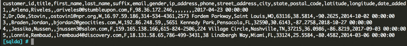
Figure 6.3: The CSV file that we created using our copy command

It is worth noting here that the formatting can look a little messy for the copy command, because it does not allow for commands with new lines. A simple way around this is to create a view containing your data before the copy command and drop the view after your copy command has finished. For example:

CREATE TEMP VIEW customers_sample AS (

    SELECT *

    FROM customers

    LIMIT 5

);

copy customers_sample TO 'my_file.csv' WITH CSV HEADER

DROP VIEW customers_sample;

While you can perform this action either way, for readability purposes, we will use the latter format in this book for longer queries.

Configuring COPY and copy

There are several options to configure the COPY and copy commands:

• FORMAT format_name can be used to specify the format. The options for format_name are csv, text, or binary. Alternatively, you can simply specify CSV or BINARY without the FORMAT keyword, or not specify the format at all and let the output default to a text file format.
• DELIMITER 'delimiter_character' can be used to specify the delimiter character for CSV or text files (for example ',' for CSV files, or '|' for pipe-separated files)
• NULL 'null_string' can be used to specify how null values should be represented (for example, ' ' if blanks represent null values, or 'NULL' if that's how missing values should be represented in the data).
• HEADER specifies that the header should be output.
• QUOTE 'quote_character' can be used to specify how fields with special characters (for example, a comma in a text value within a CSV file) can be wrapped in quotes so that they are ignored by COPY.
• ESCAPE 'escape_character' specifies the character that can be used to escape the following character.
• ENCODING 'encoding_name' allows specification of the encoding, which is particularly useful when you are dealing with foreign languages that contain special characters or user input.

Using COPY and copy to Bulk Upload Data to Your Database

As we have seen, the copy commands can be used to efficiently download data, but they can also be used to upload data.

The COPY and copy commands are far more efficient at uploading data than an INSERT statement. There are a few reasons for this:

• When using COPY, there is only one commit, which occurs after all of the rows have been inserted.
• There is less communication between the database and the client, so there is less network latency.
• Postgres includes optimizations for COPY that would not be available through INSERT.

  Here's an example of using the copy command to copy rows into the table from a file:

  copy customers FROM 'my_file.csv' CSV HEADER DELIMITER ',';

Here is the breakdown of this command and the parameters that were passed in:

• copy is invoking the Postgres COPY ... FROM STDOUT... command to load the data into the database.
• Customers specifies the name of the table that we want to append to.
• FROM 'my_file.csv' specifies that we are uploading records from my_file.csv – the FROM keyword specifies that we are uploading records as opposed to the TO keyword that we used to download records.
• The WITH CSV HEADER parameters operate the same as before.
• DELIMITER ',' specifies what the delimiter is in the file. For a CSV file, this is assumed to be a comma, so we do not need this parameter. However, for readability, it might be useful to explicitly define this parameter, for no other reason than to remind yourself how the file has been formatted.

  Note

  While COPY and copy are great for exporting data to other tools, there is additional functionality in Postgres for exporting a database backup. For these maintenance tasks, you can use pg_dump for a specific table and pg_dumpall for an entire database or schema. These commands even let you save data in compressed (tar) format, which saves space. Unfortunately, the output format from these commands is typically SQL, and it cannot be readily consumed outside of Postgres. Therefore, it does not help us with importing or exporting data to and from other analytics tools, such as Python and R.

Exercise 19: Exporting Data to a File for Further Processing in Excel

In this exercise, we will be saving a file containing the cities with the highest number of ZoomZoom customers. This analysis will help the ZoomZoom executive committee to decide where they might want to open the next dealership.

Note

For the exercises and activities in this chapter, you will need to be able to access your database with psql. https://github.com/TrainingByPackt/SQL-for-Data-Analytics/tree/master/Lesson07.

1. Open a command-line tool to implement this exercise, such as cmd for Windows or Terminal for Mac.
2. In your command-line interface, connect to your database using the psql command.
3. Copy the customers table from your zoomzoom database to a local file in .csv format. You can do this with the following command:

   CREATE TEMP VIEW top_cities AS (

       SELECT city,

              count(1) AS number_of_customers

       FROM customers

       WHERE city IS NOT NULL

       GROUP BY 1

       ORDER BY 2 DESC

       LIMIT 10

   );

   copy top_cities TO 'top_cities.csv' WITH CSV HEADER DELIMITER ','

   DROP VIEW top_cities;

   Here's a breakdown for these statements:

   CREATE TEMP VIEW top_cities AS (…) indicates that we are creating a new view. A view is similar to a table, except that the data is not created. Instead, every time the view is referenced, the underlying query is executed. The TEMP keyword indicates that the view can be removed automatically at the end of the session.

   SELECT city, count(1) AS number_of_customers … is a query that gives us the number of customers for each city. Because we add the LIMIT 10 statement, we only grab the top 10 cities, as ordered by the second column (number of customers). We also filter out customers without a city filled in.

   copy … copies data from this view to the top_cities.csv file on our local computer.

   DROP VIEW top_cities; deletes the view because we no longer need it.

   If you open the top_cities.csv text file, you should see output that looks like this:

   

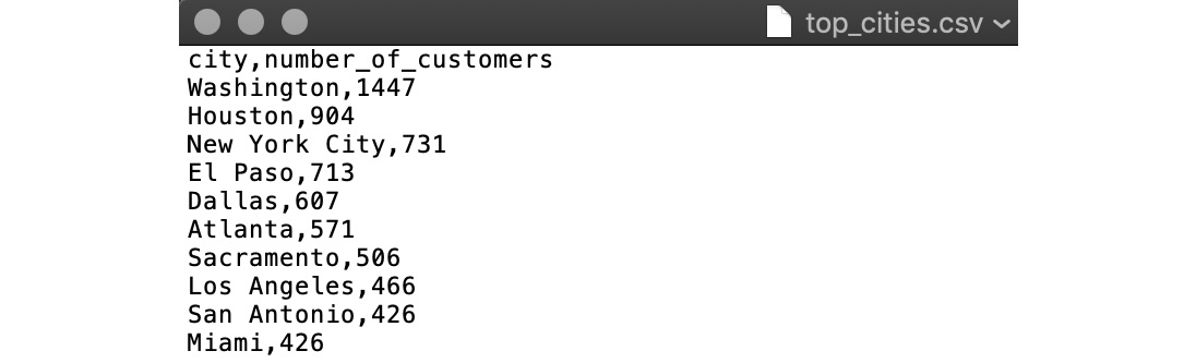
   Figure 6.4: Output from the copy command

   Note

   Here, the output file is top_cities.csv. We will be using this file in the exercises to come in this chapter.

   Now that we have the output from our database in a CSV file format, we can open it with a spreadsheet program, such as Excel.

4. Using Microsoft Excel or your favorite spreadsheet software or text editor, open the top_cities.csv file:
   

   Figure 6.5: top_cities.csv open in Excel

5. Next, select the data from cell A1 to cell B11.
   

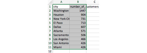
   Figure 6.6: Select the entire dataset by clicking and dragging from A1 to B11

6. Next, in the top menu, go to Insert and then click on the bar chart icon () to create a 2-D Column chart:
   

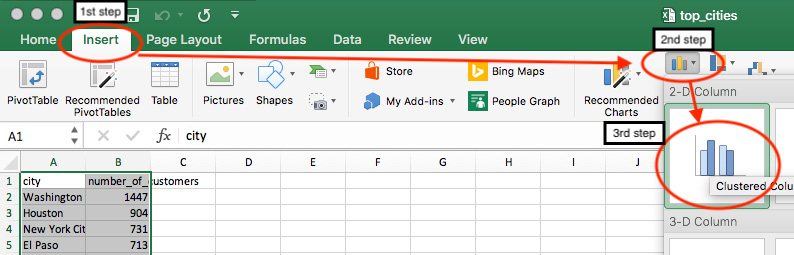
   Figure 6.7: Insert a bar chart to visualize the selected data

7. Finally, you should end up with output like this:

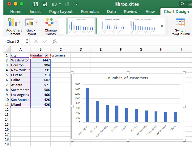
Figure 6.8: Final output from our visualization

We can see from this chart that Washington D.C. seems to have a very high number of customers. Based on this simple analysis, Washington D.C. would probably be the obvious next target for ZoomZoom expansion!

Using R with Our Database

At this point, you can now copy data to and from a database. This gives you the freedom to expand beyond SQL to other data analytics tools and incorporate any program that can read a CSV file as input into your pipeline. While just about every analytics tool that you would need can read a CSV file, there's still the extra step needed in which you download the data. Adding more steps to your analytics pipeline can make your workflow more complex. Complexity can be undesirable, both because it necessitates additional maintenance, and because it increases the number of failure points.

Another approach is to connect to your database directly in your analytics code. In this part of the chapter, we are going to look at how to do this in R, a programming language designed specifically for statistical computing. Later in the chapter, we will look at integrating our data pipelines with Python as well.

Why Use R?

While we have managed to perform aggregate-level descriptive statistics on our data using pure SQL, R allows us to perform other statistical analysis, including machine learning, regression analysis, and significance testing. R also allows us to create data visualizations that make trends clear and easier to interpret. R has arguably more statistical functionality than just about any other analytics software available.

Getting Started with R

Because R is an open source language with support for Windows, macOS X, and Linux, it is very easy to get started. Here are the steps to quickly set up your R environment:

1. Download the latest version of R from https://cran.r-project.org/.
2. Once you have installed R, you can download and install RStudio, an Integrated Development Environment (IDE) for R programming, from http://rstudio.org/download/desktop.
3. Next, we are going to install the RPostgreSQL package in R. We can do this in RStudio by navigating to the Packages tab and clicking the Install icon:
   

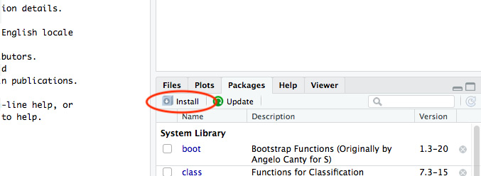
   Figure 6.9: Install R packages in RStudio in the Packages pane

4. Next, we will search for the RPostgreSQL package in the Install Packages window and install the package:
   

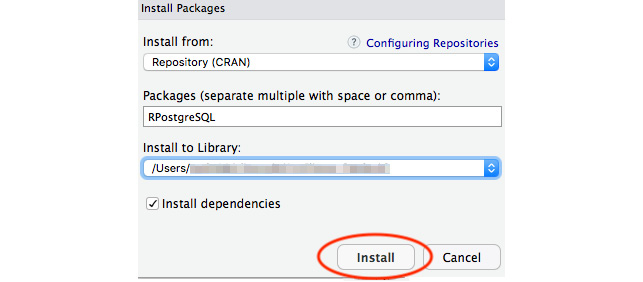
   Figure 6.10: The Install Packages prompt in RStudio allows us to search for a package

5. Next, we can use the RPostgreSQL package to load some data into R. You can use the following commands:

   library(RPostgreSQL)

   con <- dbConnect(PostgreSQL(), host="my_host", user="my_username", password="my password", dbname="zoomzoom", port=5432)

   result <- dbGetQuery(con, "select * from customers limit 10;")

   result

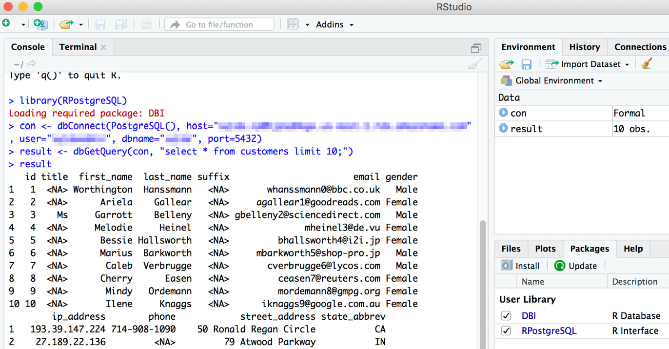
Figure 6.11: Output from our database connection in R

Here is a breakdown of these commands:

library(RPostgreSQL) is the syntax for loading a library in R.

con <- dbConnect(PostgreSQL(), host="my_host", user="my_username ", password="my_password", dbname="zoomzoom", port=5432) establishes the connection to the database. All of the database parameters are entered here, so you should replace the parameters as needed for your setup. If you have set up a .pgpass file, you can leave out the password parameter.

result <- dbGetQuery(con, "select * from customers limit 10;") is where we run a simple query to test our connection and check the result. The data is then stored in the result variable as an R dataframe.

In the last line, result is simply the name of the variable that stores our DataFrame, and the R terminal will print the contents of a variable or expression if there is no assignment.

At this point, we have successfully exported data from our database into R. This will lay the foundation for just about any analysis that you might want to perform. After you have loaded your data in R, you can continue processing data by researching other packages and techniques using other R packages. For example, dplyr can be used for data manipulation and transformation, and the ggplot2 package can be used for data visualization.

Using Python with Our Database

While R has a breadth of functionality, many data scientists and data analysts are starting to use Python. Why? Because Python offers a similarly high-level language that can be easily used to process data. While the number of statistical packages and functionality in R can still have an edge on Python, Python is growing fast, and has generally overtaken R in most of the recent polls. A lot of the Python functionality is also faster than R, in part because so much of it is written in C, a lower-level programming language.

The other large advantage that Python has is that it is very versatile. While R is generally only used in the research and statistical analysis communities, Python can be used to do anything from statistical analysis to standing up a web server. As a result, the developer community is much larger for Python. A larger development community is a big advantage because there is better community support (for example, on StackOverflow), and there are more Python packages and modules being developed every day. The last major benefit of Python is that, because it is a general programming language, it can be easier to deploy Python code to a production environment, and certain controls (such as Python namespaces) make Python less susceptible to errors.

As a result of these advantages, it might be preferable to learn Python, unless the functionality that you require is only available in R, or if the rest of your team is using R.

Why Use Python?

While SQL can perform aggregate-level descriptive statistics, Python (like R) allows us to perform other statistical analysis and data visualizations. On top of these advantages, Python can be used to create repeatable pipelines that can be deployed to production, and it can also be used to create interactive analytics web servers. Whereas R is a specialist programming language, Python is a generalist programming language – a jack of all trades. Whatever your analytics requirements are, you can almost always complete your task using the tools available in Python.

Getting Started with Python

While there are many ways to get Python, we are going to start with the Anaconda distribution of Python, which comes with a lot of the commonly used analytics packages pre-installed.

Exercise 20: Exporting Data from a Database within Python

1. Download and install Anaconda: https://www.anaconda.com/distribution/
2. Once it's installed, open Terminal for Mac or cmd for Windows. Type python on the command line, and check that you can access the Python interpreter, which should look like this:
   

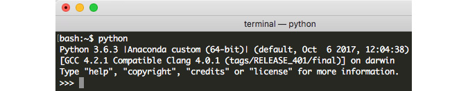
   Figure 6.12: The Python interpreter is now available and ready for input

   Note

   If you get an error, it may be because you need to specify your Python path. You can enter quit() to exit.

3. Next, we will want to install the PostgreSQL database client for Python, psycopg2. We can download and install this package using the Anaconda package manager, conda. You can enter the following command at the command line to install the Postgres database client:

   conda install psycopg2

   We can break down this command as follows:

   conda is the command for the conda package manager.

   install specifies that we want to install a new Python package.

4. Now, we can open the Python interpreter and load in some data from the database

   Type python at the command line to open the Python interpreter.

5. Next, we can start writing the Python script to load data:

   import psycopg2

   with psycopg2.connect(host="my_host", user="my_username", password="my_password", dbname="zoomzoom", port=5432) as conn:

       with conn.cursor() as cur:

           cur.execute("SELECT * FROM customers LIMIT 5")

               records = cur.fetchall()

   records

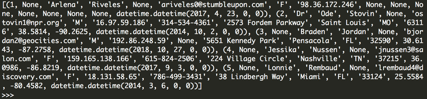
Figure 6.13: Output from our database connection in Python

These commands can be broken down as follows:

First, we import the psycopg2 package using the following command: import psycopg2. Next, we set up our connection object using psycopg2.connect(host="my_host", user="my_username", password="my_password", dbname="zoomzoom", port=5432).

All of the database parameters are entered here, so you should replace the parameters as required for your setup. If you have set up a .pgpass file, you can leave out the password parameter. This is wrapped in with .. as conn in Python; the with statement automatically tears down the object (in this case, the connection) when the indentation returns. This is particularly useful for database connection, where an idle connection could inadvertently consume database resources. We can store this connection object in a conn variable using the as conn statement.

Now that we have a connection, we need to create a cursor object, which will let us read from the database. conn.cursor() creates the database cursor object, which allows us to execute SQL in the database connection, and the with statement allows us to automatically tear down the cursor when we no longer need it.

cur.execute("SELECT * FROM customers LIMIT 5") sends the query "SELECT * FROM customers LIMIT 5" to the database and executes it.

records = cur.fetchall() fetches all of the remaining rows in a query result and assigns those rows to the records variable.

Now that we have sent the query to the database and received the records, we can reset the indentation level. We can view our result by entering the expression (in this case, just the variable name records) and hitting Enter. This output is the five customer records that we have collected.

While we were able to connect to the database and read data, there were several steps, and the syntax was a little bit more complex than that for some of the other approaches we have tried. While psycopg2 can be powerful, it can be helpful to use some of the other packages in Python to facilitate interfacing with the database.

Improving Postgres Access in Python with SQLAlchemy and Pandas

While psycopg2 is a powerful database client for accessing Postgres from Python, we can simplify the code by using a few other packages, namely, Pandas and SQLAlchemy.

First, we will look at SQLAlchemy, a Python SQL toolkit and object relational mapper that maps representations of objects to database tables. In particular, we will be looking at the SQLAlchemy database engine and some of the advantages that it offers. This will enable us to access our database seamlessly without worrying about connections and cursors.

Next, we can look at Pandas – a Python package that can perform data manipulation and facilitate data analysis. The pandas package allows us to represent our data table structure (called a DataFrame) in memory. Pandas also has high-level APIs that will enable us to read data from our database in just a few lines of code:

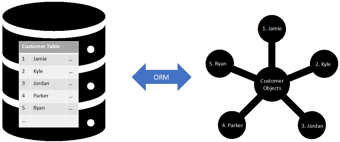
Figure 6.14: An object relational mapper maps rows in a database to objects in memory

While both of these packages are powerful, it is worth noting that they still use the psycopg2 package in order to connect to the database and execute queries. The big advantage that these packages provide is that they abstract some of the complexities of connecting to the database. By abstracting these complexities, we can connect to the database without worrying that we might forget to close a connection or tear down a cursor.

What is SQLAlchemy?

SQLAlchemy is a SQL toolkit. While it offers some great functionality, the key benefit that we will focus on here is the SQLAlchemy Engine object.

A SQLAlchemy Engine object contains information about the type of database (in our case, PostgreSQL) and a connection pool. The connection pool allows for multiple connections to the database that operate simultaneously. The connection pool is also beneficial because it does not create a connection until a query is sent to be executed. Because these connections are not formed until the query is being executed, the Engine object is said to exhibit lazy initialization. The term "lazy" is used to indicate that nothing happens (the connection is not formed) until a request is made. This is advantageous because it minimizes the time of the connection and reduces the load on the database.

Another advantage of the SQLAlchemy Engine is that it automatically commits (autocommits) changes to the database due to CREATE TABLE, UPDATE, INSERT, or other statements that modify our database.

In our case, we will want to use it because it provides a robust Engine to access databases. If the connection is dropped, a SQLAlchemy Engine can instantiate that connection because it has a connection pool. It also provides a nice interface that works well with other packages (such as pandas).

Using Python with Jupyter Notebooks

In addition to interactively using Python at the command line, we can use Python in a notebook form in our web browser. This is useful for displaying visualizations and running exploratory analyses.

In this section, we are going to use Jupyter notebooks that were installed as part of the Anaconda installation. At the command line, run the following command:

jupyter notebook

You should see something like this pop up in your default browser:

Figure 6.15: Jupyter notebook pop-up screen in your browser

Next, we will create a new notebook:

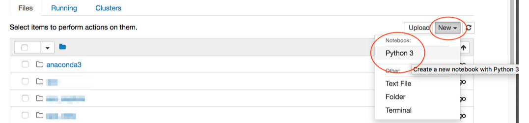
Figure 6.16: Opening a new Python 3 Jupyter notebook

At the prompt, enter the following import statements:

from sqlalchemy import create_engine

import pandas as pd

You'll notice that we are importing two packages here – the first is the create_engine module within the sqlalchemy package, and the second is pandas, which we rename to pd because this is the standard convention (and it is fewer characters). Using these two packages, we will be able to read and write data to and from our database and visualize the output.

Hit Shift+Enter to run these commands. A new active cell should pop up:

Figure 6.17: Running our first cell in the Jupyter notebook

Next, we will configure our notebook to display plots and visualizations inline. We can do this with the following command:

% matplotlib inline

This tells the matplotlib package (which is a dependency of pandas) to create plots and visualizations inline in our notebook. Hit Shift + Enter again to jump to the next cell.

In this cell, we will define our connection string:

cnxn_string = ("postgresql+psycopg2://{username}:{pswd}"

               "@{host}:{port}/{database}")

print(cnxn_string)

Press Shift + Enter again, and you should now see our connection string printed. Next, we need to fill in our parameters and create the database Engine. You can replace the strings starting with your_ with the parameters specific to your connection:

engine = create_engine(cnxn_string.format(

    username="your_username",

    pswd="your_password",

    host="your_host",

    port=5432,

    database="your_database_name"))    

In this command, we run create_engine to create our database Engine object. We pass in our connection string and we format it for our specific database connection by filling in the placeholders for {username}, {pswd}, {host}, {port}, and {database}.

Because SQLAlchemy is lazy, we will not know whether our database connection was successful until we try to send a command. We can test whether this database Engine works by running the following command and hitting Shift + Enter:

engine.execute("SELECT * FROM customers LIMIT 2;").fetchall()

We should see something like this:

Figure 6.18: Executing a query within Python

The output of this command is a Python list containing rows from our database in tuples. While we have successfully read data from our database, we will probably find it more practical to read our data into a Pandas DataFrame in the next section.

Reading and Writing to our Database with Pandas

Python comes with great data structures, including lists, dictionaries, and tuples. While these are useful, our data can often be represented in a table form, with rows and columns, similar to how we would store data in our database. For these purposes, the DataFrame object in Pandas can be particularly useful.

In addition to providing powerful data structures, Pandas also offers:

• Functionality to read data in directly from a database
• Data visualization
• Data analysis tools

If we continue from where we left off with our Jupyter notebook, we can use the SQLAlchemy Engine object to read data into a Pandas DataFrame:

customers_data = pd.read_sql_table('customers', engine)

We have now stored our entire customers table as a Pandas DataFrame in the customers_data variable. The Pandas read_sql_table function requires two parameters: the name of a table and the connectable database (in this case, the SQLAlchemy Engine). Alternatively, we can use the read_sql_query function, which takes a query string instead of a table name.

Here's an example of what your notebook might look like at this point:

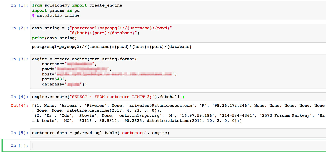
Figure 6.19: The entirety of our Jupyter notebook

Performing Data Visualization with Pandas

Now that we know how to read data from the database, we can start to do some basic analysis and visualization.

Exercise 21: Reading Data and Visualizing Data in Python

In this exercise, we will be reading data from the database output and visualizing the results using Python, Jupyter notebooks, SQLAlchemy, and Pandas. We will be analyzing the demographic information of customers by city to better understand our target audience.

1. Open the Jupyter notebook from the previous section and click on the last empty cell.
2. Enter the following query surrounded by triple quotes (triple quotes allow for strings that span multiple lines in Python):

   query = """

       SELECT city,

              COUNT(1) AS number_of_customers,

              COUNT(NULLIF(gender, 'M')) AS female,

              COUNT(NULLIF(gender, 'F')) AS male

       FROM customers

       WHERE city IS NOT NULL

       GROUP BY 1

       ORDER BY 2 DESC

       LIMIT 10

   """

   For each city, this query calculates the count of customers, and calculates the count for each gender. It also removes customers with missing city information and aggregates our customer data by the first column (the city). In addition, it sorts the data by the second column (the count of customers) from largest to smallest (descending). Then, it limits the output to the top 10 (the 10 cities with the highest number of customers).

3. Read the query result into a Pandas DataFrame with the following command and execute the cells using Shift + Enter:

   top_cities_data = pd.read_sql_query(query, engine)

4. You can view the data in top_cities_data by entering it in a new cell and simply hitting Shift + Enter. Just as with the Python interpreter, entering a variable or expression will display the value. You will notice that Pandas also numbers the rows by default – in Pandas, this is called an index.
   

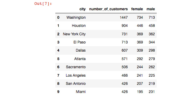
   Figure 6.20: storing the result of a query as a pandas dataframe

5. Now, we will plot the number of men and women in each of the top 10 cities. Because we want to view the stats for each city separately, we can use a simple bar plot to view the data:

   ax = top_cities_data.plot.bar('city', y=['female', 'male'], title='Number of Customers by Gender and City')

   Here is a screenshot of what our resulting output notebook should look like:

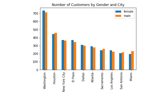
Figure 6.21: Data visualization in the Jupyter notebook

The results show that there is no significant difference in customer gender for the cities that we are considering expanding into.

Writing Data to the Database Using Python

There will also be many scenarios in which we will want to use Python to write data back to the database, and, luckily for us, Pandas and SQLAlchemy make this relatively easy.

If we have our data in a Pandas DataFrame, we can write data back to the database using the Pandas to_sql(…) function, which requires two parameters: the name of the table to write to and the connection. Best of all, the to_sql(…) function also creates the target table for us by inferring column types using a DataFrame's data types.

We can test out this functionality using the top_cities_data DataFrame that we created earlier. Let's use the following to_sql(…) command in our existing Jupyter notebook:

top_cities_data.to_sql('top_cities_data', engine,

                       index=False, if_exists='replace')

In addition to the two required parameters, we added two optional parameters to this function – the index parameter specifies whether we want the index to be a column in our database table as well (a value of False means that we will not include it), and the if_exists parameter allows us to specify how to handle a scenario in which there is already a table with data in the database. In this case, we want to drop that table and replace it with the new data, so we use the 'replace' option. In general, you should exercise caution when using the 'replace' option as you can inadvertently lose your existing data.

Now, we can query this data from any database client, including psql. Here is the result when we try to query this new table in our database:

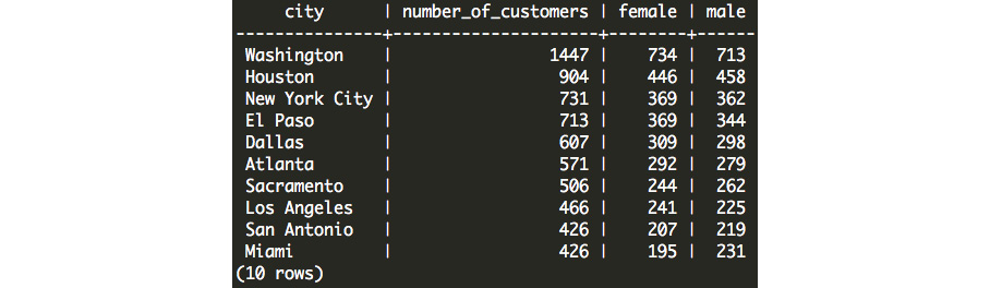
Figure 6.22: Data created in Python that has now been imported into our database

Improving Python Write Speed with COPY

While this functionality is simple and works as intended, it is using insert statements to send data to the database. For a small table of 10 rows, this is OK, but for larger tables, the psql copy command is going to be much faster.

We can actually use the COPY command in conjunction with Python, SQLAlchemy, and Pandas to deliver the same speed that we get with copy. Say we define the following function:

import csv

from io import StringIO

def psql_insert_copy(table, conn, keys, data_iter):

    # gets a DBAPI connection that can provide a cursor

    dbapi_conn = conn.connection

    with dbapi_conn.cursor() as cur:

        s_buf = StringIO()

        writer = csv.writer(s_buf)

        writer.writerows(data_iter)

        s_buf.seek(0)

        columns = ', '.join('"{}"'.format(k) for k in keys)

        if table.schema:

            table_name = '{}.{}'.format(table.schema, table.name)

        else:

            table_name = table.name

        sql = 'COPY {} ({}) FROM STDIN WITH CSV'.format(

            table_name, columns)

        cur.copy_expert(sql=sql, file=s_buf)

We can then leverage the method parameter in to_sql, as shown here:

top_cities_data.to_sql('top_cities_data', engine,

                       index=False, if_exists='replace',

                       method=psql_insert_copy)

The psql_insert_copy function defined here can be used without modification in any of your PostgreSQL imports from Pandas. Here is a breakdown of what this code does:

1. After performing some necessary imports, we begin by defining the function using the def keyword followed by the function name (psql_insert_copy) and the parameters (table, conn, keys, and data_iter).
2. Next, we establish a connection (dbapi_conn) and cursor (cur) that we can use for execution.
3. Next, we write all of the data in our rows (represented in data_iter) to a string buffer (s_buf) that is formatted like a CSV file, but that exists in memory and not in a file on our hard drive.
4. Then, we define the column names (columns) and table name (table_name).
5. Lastly, we execute the COPY statement by streaming the CSV file contents through Standard input (STDIN).

Reading and Writing CSV Files with Python

In addition to reading and writing data to our database, we can use Python to read and write data from our local filesystem. The commands for reading and writing CSV files with Pandas are very similar to those used for reading and writing from our database:

For writing, pandas.DataFrame.to_csv(file_path, index=False) would write the DataFrame to your local filesystem using the supplied file_path.

For reading, pandas.read_csv(file_path, dtype={}) would return a DataFrame representation of the data supplied in the CSV file located at file_path.

When reading a CSV file, Pandas will infer the correct data type based on the values in the file. For example, if the column contains only integer numbers, it will create the column with an int64 data type.

Similarly, it can infer whether a column contains floats, timestamps, or strings. Pandas can also infer whether or not there is a header for the file, and generally, this functionality works pretty well. If there is a column that is not read in correctly (for example, a five-digit US zip code might get read in as an integer causing leading zeros to fall off – "07123" would become 7123 without leading zeros), you can specify the column type directly using the dtype parameter. For example, if you have a zip_code column in your dataset, you could specify that it is a string using dtype={'zip_code': str}.

Note

There are many different ways in which a CSV file might be formatted. While pandas can generally infer the correct header and data types, there are many parameters offered to customize the reading and writing of a CSV file for your needs.

Using the top_cities_data in our notebook, we can test out this functionality:

top_cities_data.to_csv('top_cities_analysis.csv', index=False)

my_data = pd.read_csv('top_cities_analysis.csv')

my_data

my_data now contains the data that we wrote to a CSV and then read it back in. We do not need to specify the optional dtype parameter in this case because our columns could be inferred correctly using pandas. You should see an identical copy of the data that is in top_cities_data:

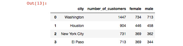
Figure 6.23: Checking that we can write and read CSV files in pandas

Best Practices for Importing and Exporting Data

At this point, we have seen several different methods for reading and writing data between our computer and our database. Each method has its own use case and purpose. Generally, there are going to be two key factors that should guide your decision-making process:

• You should try to access the database with the same tool that you will use to analyze the data. As you add more steps to get your data from the database to your analytics tool, you increase the ways in which new errors can arise. When you can't access the database using the same tool that you will use to process the data, you should use psql to read and write CSV files to your database.
• When writing data, you can save time by using the COPY or copy commands.

Going Password-Less

In addition to everything mentioned so far, it is also a good idea to set up a .pgpass file. A .pgpass file specifies the parameters that you use to connect to your database, including your password. All of the programmatic methods of accessing the database discussed in this chapter (using psql, R, and Python) will allow you to skip the password parameter if your .pgpass file contains the password for the matching hostname, database, and username.

On Unix-based systems and macOS X, you can create the .pgpass file in your home directory. On Windows, you can create the file in %APPDATA%postgresqlpgpass.conf. The file should contain one line for every database connection that you want to store, and it should follow this format (customized for your database parameters):

hostname:port:database:username:password

For Unix and Mac users, you will need to change the permissions on the file using the following command on the command line (in the Terminal):

chmod 0600 ~/.pgpass

For Windows users, it is assumed that you have secured the permissions of the file so that other users cannot access it. Once you have created the file, you can test that it works by calling psql as follows in the terminal:

psql -h my_host -p 5432 -d my_database -U my_username

If the .pgpass file was created successfully, you will not be prompted for your password.

Activity 8: Using an External Dataset to Discover Sales Trends

In this activity, we are going to use United States Census data on public transportation usage by zip code to see whether the level of use of public transport has any correlation to ZoomZoom sales in a given location.

1. Download the public transportation according to zip code dataset from GitHub:

   https://github.com/TrainingByPackt/SQL-for-Data-Analytics/blob/master/Datasets/public_transportation_statistics_by_zip_code.csv

   This dataset contains three columns:

   zip_code: This is the five-digit United States postal code that is used to identify the region.

   public_transportation_pct: This is the percentage of the population in a postal code that has been identified as using public transportation to commute to work.

   public_transportation_population: This is the raw number of people in a zip code that use public transportation to commute to work.

2. Copy the data from the public transportation dataset to the ZoomZoom customer database by creating a table for it in the ZoomZoom dataset.
3. Find the maximum and minimum percentages in this data. Values below 0 will most likely indicate missing data.
4. Calculate the average sales amounts for customers that live in high public transportation regions (over 10%) as well as low public transportation usage (less than, or equal to, 10%).
5. Read the data into pandas and plot a histogram of the distribution (hint: you can use my_data.plot.hist(y='public_transportation_pct') to plot a histogram if you read the data into a my_data pandas DataFrame).
6. Using pandas, test using the to_sql function with and without the method=psql_insert_copy parameter. How do the speeds compare? (Hint: In a Jupyter notebook, you can add %time in front of your command to see how long it takes.)
7. Group customers based on their zip code public transportation usage, rounded to the nearest 10%, and look at the average number of transactions per customer. Export this data to Excel and create a scatterplot to better understand the relationship between public transportation usage and sales.
8. Based on this analysis, what recommendations would you have for the executive team at ZoomZoom when considering expansion opportunities?

   Note

   The solution to this activity can be found on page 328.

Summary

In this chapter, we learned how to interface our database with other analytical tools for further analysis and visualization. While SQL is powerful, there are always going to be some analyses that need to be undertaken in other systems and being able to transfer data in and out of the database enables us to do just about anything we want with our data.

In the next chapter, we will examine data structures that can be used to store complex relationships in our data. We will learn how to mine insights from text data, as well as look at the JSON and ARRAY data types so that we can make full use of all of the information available to us.