
9
AgentFly: Scalable, High-Fidelity Framework for Simulation, Planning and Collision Avoidance of Multiple UAVs
David Šišlák, P![]() emysl Volf, Št
emysl Volf, Št![]() pán Kop
pán Kop![]() iva and Michal P
iva and Michal P![]() chou
chou![]() ek
ek
AgentFly is a software prototype providing intelligent algorithms for autonomous unmanned aerial vehicles. AgentFly is implemented as a scalable multi-agent system in JAVA running on the top of the Aglobe platform [1] which provides flexible middle-ware supporting seamless interaction among heterogenous software, hardware and human actors. Thanks to JAVA, AgentFly can easily be hosted on UAVs or computers with different operating systems. The multi-agent approach [2] provides straightforward mapping – each airplane is controlled by one agent. Agents integrate intelligent algorithms providing a coordination-based control for autonomous UAVs. In the presented work, only algorithms which are fully distributed among airplanes are used. Such algorithms provide a real autonomous control for UAVs which do not require any central unit (a ground station or master airplane) controlling a group of UAVs. The main benefit is that the group of UAVs can also operate in situations where the permanent communication link with the central unit or ground operating station is missing. Some of the algorithms presented in this chapter suppose that UAVs are equipped with communication modems which allow them to dynamically establish bi-directional communication channels based on their mutual position. Thus, airplanes utilize the mobile ad-hoc wireless network [3] created by their communication modems. These algorithms provide robust control in critical situations: loss of communication, destroyed airplane.
The AgentFly system has been developed over more than five years. It was initially built for simulation-based validation and comparison of various approaches for autonomous collision avoidance algorithms adopting the free-flight concept [4]. Later, AgentFly was extended with a high-level control providing tactical control team coordination. Even though the AgentFly system has been developed primarily for simulation purposes, the same agents and algorithms are also deployed for real UAV platforms. Beside UAV application, the US Federal Aviation Administration (FAA) supports the application of the AgentFly system for simulation and evaluation of the future civilian air-traffic management system which is being studied within the large research program called Next Generation Air Transportation Systems (NGATS) [5]. AgentFly has been extended with high-fidelity models of civilian airplanes and to support a human-based air-traffic control. The current version of AgentFly is suitable for several use-case models: a tool for empirical analysis, an intelligent control for UAVs and hybrid simulations. The hybrid simulation allows us to integrate a real flying UAV platform into a virtual situation and perform initial validation of algorithms in hazardous situations (which could be very expensive while done only with real platforms) and also perform scalability evaluation of intelligent algorithms with thousands of UAVs.
The rest of the chapter is organized as follows. Section 9.1 presents the overall multi-agent architecture of AgentFly. Section 9.2 describes the extensible layered UAV control concept. Section 9.3 briefly introduces algorithms used in the trajectory planning component and their comparison to other existing state-of-the-art methods. Section 9.4 describes the multi-layer collision avoidance framework providing the sense and avoid capability to an airplane. Section 9.5 provides the description of existing high-level coordination algorithms integrated with AgentFly. Section 9.6 presents distribution and scalability of the AgentFly simulation with respect to the number of UAVs. Finally, Section 9.7 documents the deployment of the AgentFly system and included algorithms to the real UAV platform.
9.1 Agent-Based Architecture
All components in AgentFly are implemented as software agents in the multi-agent middle-ware Aglobe [1]. Aglobe is like an operating system providing run-time environment for agents. It provides agent encapsulation, efficient agent-to-agent communication, high-throughput message passing with both address-determined and content-determined receivers, yellow page services providing the address look-up function, migration support, and also agent life-cycle management. The Aglobe platform has been selected because it outperforms other existing multi-agent platforms with its limited computational resources and very efficient operation. Moreover, Aglobe facilitates modeling of communication inaccessibility and unreliability in ad-hoc networking environments.
The high-level overview of the AgentFly agent-based architecture is shown in Figure 9.1. Basically, there exist three different types of agent in AgentFly: (i) UAV agents, (ii) environmental simulation agents, and (iii) visio agents. When AgentFly is started in the simulation mode, usually all three types of agent are used. On the other hand, when AgentFly is running directly on a real UAV platform, only UAV agents are running (one UAV agent per UAV platform) and an actuator control and sensing perceptions are mapped to real hardware.
Figure 9.1 AgentFly system structure overview
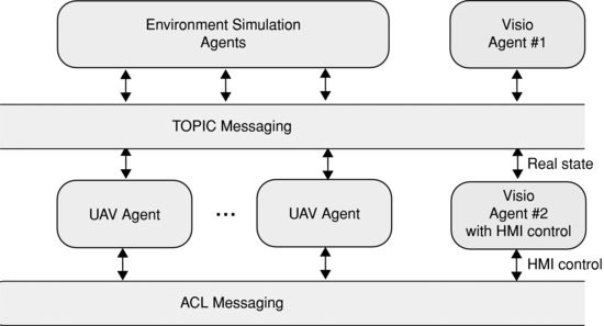
9.1.1 UAV Agents
Each UAV in AgentFly is represented by one UAV agent. This agent provides the unit control for UAV. Intelligent algorithms for UAVs are integrated in this agent. Based on the configuration, they provide high-level functions like trajectory planning, collision avoidance, see and avoid functionality, and also autonomous coordination of a group of UAVs. AgentFly usually integrates algorithms providing a decentralized control approach. Thus, appropriate parts of algorithms are running in a distributed manner within several UAV agents and they can utilize ACL messaging providing UAV-to-UAV communication channels. If it is required by the experimental setup to use an algorithm which needs some centralized component, another agent can be created which is not tightly bound with any specific UAV.
9.1.2 Environment Simulation Agents
Environment simulation agents are used when AgentFly is started in the simulation mode. These agents are responsible for simulation of a virtual environment in which UAVs are operated. These agents replace actions which normally happen in the real world. They provide simulation of physical behaviors of virtual UAVs (non-real UAV platforms), mutual physical interactions (physical collisions of objects), atmospheric model (weather condition) influencing UAV behavior, communication parameters based on the used wireless simulator, and simulation of non-UAV entities in the scenario (e.g. humans, ground units). Through simulation infrastructure, these agents provide sensing perceptions for UAV agents. Beside simulation, there exist simulation control agents which are responsible for the scenario control (initialization of entities, parameter setups, etc.) and for data acquisition and analysis of configured properties which are studied in a scenario. These agents are created so that they support large-scale simulations that are distributively started over several computers connected by a network, see Section 9.6 for details.
9.1.3 Visio Agents
Visio agents provide real-time visualization of the internal system state in a 3D or 2D environment. Based on a configuration, much UAV-related information can also be displayed in various ways. In AgentFly, several visio agents providing the same or different presentation layers from various perspectives can be connected simultaneously. The architecture of AgentFly automatically optimizes data collection and distribution so that the network infrastructure is optimally utilized. A visio agent can be configured to provide HMI for the system, e.g. the user operator can amend the goal for algorithms.
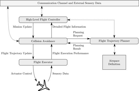
Figure 9.2 The UAV’s control architecture: control blocks and their interactions
9.2 Airplane Control Concept
The AgentFly UAV control concept uses the layered control architecture, see Figure 9.2. Many common collision avoidance approaches widely used in the research community [6--13] provide control based on a direct change of the appropriate airplane’s state, e.g. a heading change control. Such control methods don’t provide a straightforward way for complex deliberative UAV control because there is no detailed information about the future flight which is necessary for selection of the suitable solution from several versions. For example, the set of tasks should be fulfilled as soon as possible by a group of UAVs. Due to the lack of detailed flight information, a task controller cannot assign tasks to UAVs with respect to the required time criterion. The method used in AgentFly is based on a complete flight trajectory description. The flight trajectory is the crucial structure which provides a description of future UAV intentions, covering also the uncertainty while they are executed by UAVs. In AgentFly, it is supposed that UAVs operate in a shared limited three-dimensional airspace called the operation space. Additional limits of the operation space are given by separation from the ground surface and by a set of no-flight areas which define a prohibited space for UAVs. No-flight areas are also known as special use airspaces (SUAs) in civilian air-traffic [14]. These no-flight areas can be dynamically changed during the run-time (e.g. there is identified an air defense patrol by an other UAV). Beside the flight trajectory, another crucial structure called the mission is used. The mission is an ordered sequence of waypoints, where each waypoint can specify geographical and altitude constraints and combine optional constraints: time restrictions (e.g. not later than, not earlier than), a fly speed restriction, and an orientation restriction.
The flight control in AgentFly is decomposed into several components, as shown in Figure 9.2:
- Flight executor – The flight executor holds the current flight trajectory which is executed (along which the UAV is flying). The flight executor implements an autopilot function in order to track the request intentions in a flight trajectory as precisely as possible. Such intelligent autopilot is known as the flight management system (FMS) [15] in civilian airplanes. The flight executor is connected to many sensors and to all available actuators which are used to control the flight of a UAV platform.
Based on current aerometric values received from an airplane’s flight sensors and the required flight trajectory, the autopilot provides control for UAV actuators. Aerometric data include the position (e.g. from the global positioning system (GPS) or inertial navigation system (INS)), the altitude from a barometric altimeter, the pressure-based airspeed and attitude sensors providing an angular orientation of UAV from gyroscopes. Depending on the UAV construction, the following primary actuators can be used: ailerons (rotation around longitudinal axis control), elevators (rotation around lateral axis control), rudder (compensation of g-forces), and thrust power (engine speed control). Large UAVs can also be equipped with secondary actuators changing their flight characteristics: wing flaps, slats, spoilers, or air brakes.
The design of the flight executor (autopilot) is tightly coupled with the UAV airframe construction and its parameters. Its design is very complex and is not in the scope of this chapter. The control architecture covers the varying flight characteristics which are primarily affected by changing atmospheric conditions (e.g. the wind direction and speed). The control architecture supposes that the flight trajectory is executed within a defined horizontal and vertical tolerance. These tolerances cover the precision of sensors and also imprecise flight execution. The flight executor is aware of these tolerances and provides the current flight precision in its output. Section 9.7 includes the description of AgentFly deployment to the Procerus UAV platform.
The current flight execution performance is monitored by layers above the flight executor and if it is out of the predicted one included in the executed flight trajectory, the replanning process is invoked. This is how AgentFly works with the position-based uncertainty present in the real UAV platform. - Flight trajectory planner – The flight trajectory planner is the sole component in the UAV control architecture which is responsible for the creation of all flight trajectories. Planning can be viewed as the process of transformation of a waypoint sequence to the detailed flight intent description considering UAV model restrictions (flight dynamics) and the airspace definition. More information about the flight trajectory planner is provided in Section 9.3.
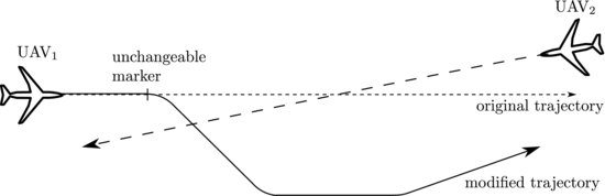
Beside planning (which is usually used only before the UAV is started), it is also capable of replanning (modification of an existing flight trajectory). In the case of replanning, the planning request contains the unique identifier of the position from which the plan has to be modified. This unique identifier is known as the unchangeable marker. Existence of the unchangeable marker in replanning is necessary for the case when a UAV is already flying and wants to change its currently executed flight trajectory. All intelligent algorithms used for UAV control run in non-zero time based on their complexity. Moreover, while the replanning process is running, the UAV is still flying. The flight trajectory can be changed only in the future, otherwise it is not accepted by the flight executor (as it is not consistent with the current UAV state, including its position). It can happen that for a planning request (an unchangeable marker and waypoint sequence) the planner is not able to provide a flight trajectory (e.g. a waypoint lies outside the operational airspace or it cannot satisfy any optional constraints). In such a case, the flight trajectory planner returns a failure as the planning result. - Collision avoidance – The collision avoidance component is responsible for implementation of the sense and avoid function for a UAV. In AgentFly, the method using additional control waypoints which are inserted into the current mission waypoint sequence is used. These control waypoints are injected so that the final trajectory is collision-free with respect to other UAVs or piloted airplanes operating in the same airspace. The collision avoidance component chooses the appropriate collision modification with respect to the selected airplane preferences and optimization criterion. Each such considered modification is transformed in the flight trajectory utilizing the flight trajectory planner.
Algorithms for collision avoidance in AgentFly implemented by the Agent Technology Center utilize the decentralized approach based on the free-flight concept [4] – the UAV can fly freely according to its own priority but still respects the separation requirements from others in its neighborhood. This means there is no centralized element responsible for providing collision-free flight trajectories for UAVs operating in the same shared airspace. Intelligent algorithms integrated in this component can utilize a communication channel provided by onboard wireless data modems and sensory data providing information about objects in its surrounding (a large UAV platform can be equipped with an onboard radar system, a smaller one can utilize receivers of transponders’ replies or receives radar-like data from a ground/AWACS radar system).
Collision avoidance implements the selected flight plan by passing the flight trajectory update to the flight executor. Collision avoidance utilizes the flight execution performance (uncertainty in the flight execution) to adjust the algorithm separation used while searching for a collision-free trajectory for the UAV. Collision avoidance monitors modification of the UAV mission coming from the upper layer and also detects execution performance beyond that predicted in the currently executed flight trajectory. In such a case, collision avoidance invokes replanning with new tolerances and conflict detection and separation processes are restarted with the new condition. More details about collision avoidance algorithms in AgentFly are provided in Section 9.4. - High-level flight controller – The high-level flight controller provides a goal-oriented control for UAVs. This component includes intelligent algorithms for the group coordination and team action planning (assignment of the specific task to the particular UAV). Depending on the configured algorithm, the high-level flight controller utilizes the communication channel, sensory perceptions (e.g. preprocessed camera inputs), and the flight trajectory planner to decide which tasks should be done by the UAV. Tasks for the UAV are then formulated as a mission which is passed to the collision avoidance component. During the flight, the high-level flight controller receives updates with the currently executed flight trajectory, including modification caused by collision avoidance. The high-level flight controller can identify that properties of the flight trajectory are no longer sufficient for the current tasks. In such a case, the high-level flight controller invokes algorithms to renegotiate and adjust task allocations for UAVs and thus modify the current UAV mission. Examples of high-level flight control algorithms are given in Section 9.5.
If no high-level algorithm is used, a simple implementation of this component can be made which just provides one initial flight mission for the UAV composed as a sequence of waypoints from a departing position, flight fixes (where the UAV should fly through), and a destination area where it has to land.
9.3 Flight Trajectory Planner
The flight trajectory planner is a very important component in the control architecture presented in the previous section. It is the only component which is responsible for preparation of the flight trajectory for a UAV. Any time when other components require preparing a new version of the flight trajectory they call the planner with an appropriate planning request containing an unchangeable marker and waypoint sequence. The efficiency of this component has influence on the overall system performance. For example, while an intelligent algorithm searches for an optimal solution for an identified collision among UAVs, the planner can be called many times even though finally only one trajectory is selected and applied for its execution. Such a mechanism allows other layers to evaluate various flight trajectories considering their feasibility, quality, and also with respect to the future waypoint constraints. Similarly, the high-level flight controller can call the planner many times while it evaluates task assignments. The planner should be fast enough. There exist many trajectory approaches known from the robotics planning domain. There is a trade-off between optimality of the path planner and its performance.
AgentFly uses the optimization-based flight trajectory planner based on the classical A* algorithm [16]. The planner searches for the valid three-dimensional flight trajectory which has the minimum cost for a given criterion function. The search in the continuous space is transformed to the search within a dynamically generated state space where states are generated by UAV motion elements based on its model. The flight trajectory has to respect all dynamic constraints specified for the UAV model the trajectory has to be smooth (smooth turns), limits and acceleration in flight speed, etc. There is defined a set of possible control modes (flight elements) for the UAV which covers the whole maneuverability of the UAV. The basic set consists of straight, horizontal turn, vertical turn, and spiral elements. These elements can be combined together and are parameterized so that a very rich state space can be generated defining UAV motion in the continuous three-dimensional space. The example of generation of samples in two-dimensional space is shown in Figure 9.3. Us of the original A* algorithm is possible over this dynamically generated state space but its performance is very limited by the size of a state space rapidly growing with the size of the operation space for the UAV.
Figure 9.3 An example of generation of new samples from the current planning configuration in two-dimensional space
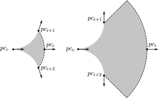
Figure 9.4 An example of adaptive sampling in two-dimensional space
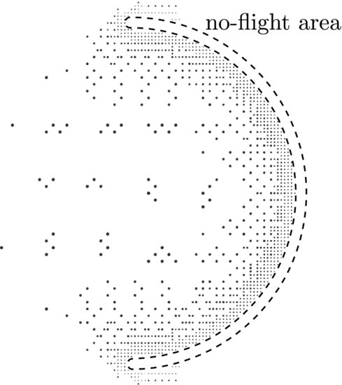
In order to improve performance of the search, the Accelerated A* (AA*) algorithm has been developed [17]. The simplified pseudo-code of the AA* algorithm is provided in Algorithm 9.1. AA* extends the original A* algorithm to be usable in large-scale environments while still providing a certain level of search precision. AA* removes the trade-off between the speed and search precision by the introduction of adaptive sampling – parameters used for generating elements are determined based on the distance to the nearest obstacle (operating space boundary or no-flight area). If the state is far from any obstacle, parameters are higher and thus produce longer flight elements and vice versa. This adaptive parameterization is included in each state while it is generated (line 9). Sampling parameterization is then used within the Expand function (line 7). Adaptive sampling leads to variable density of samples, see Figure 9.4 – samples are sparse far from obstacles and denser when they are closer.
Algorithm 9.1 The AA* algorithm pseudo-code.

Adaptive sampling in AA* requires a similarity test instead of a equality test over OPEN and CLOSED lists while a new state is generated (lines 11 and 14). Because of the adaptive sampling step, usage of the equality test will lead to a high number of states, leading to a high density of states in areas far from any no-flight area. This is caused by the fact that generation is not the same in the reverse direction because those states typically have different sampling parameters due to different distances to the nearest no-flight areas. AA* uses sampling parameters based on the power of two multiplied by the search precision (minimum sampling parameters). Two states are treated as similar if their distance is less than half the sampling step. The algorithm is more complex as it also consider different orientations within the state, see [17] for details.
The path constructed as a sequence of flight elements can be curved more than is necessary due to the sampling mechanism described above. To remove this undesired feature of the planner, each path candidate generated during the search (line 13) is smoothed. Smoothing in AA* is the process of finding a new parent for the state for which the cost of the path from the start to the current state is lower than the cost of the current path via the original state parent. Such a parent candidate is searched for among all the states from CLOSED. The parent replacement can be accepted only if a new trajectory goes only within the UAV operating space and respects all constraints defined by its flight dynamics.
Figure 9.5 Any-angle path planning in the grid
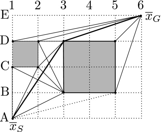
Properties of the AA* algorithm have been studied and compared with existing state-of-the-art planning methods using the modified search domain which is common to many algorithms. The modified domain is known as any-angle grid-based planning [18], see Figure 9.5. In such a planning problem, connection of any two vertices is allowed if the connecting line doesn’t intersect any blocked cell. This problem is close to the planning described above. Two-dimensional any-angle planning can be viewed as planning for a UAV which is restricted to fly at one altitude and the horizontal turn radius is limited to zero. This means that the UAV can turn (change its horizontal orientation) without any transition. For this reduced planning problem, there is provided a mathematical analysis of AA* sub-optimality. The result proves that all solutions provided by the AA* algorithm are always within a certain tolerance from the optimal solutions. The sub-optimality range can be uniquely derived from the grid configuration, see [19] for details.
Several existing planning algorithms were selected, and used for comparison with AA*: the original A* algorithm [16] adapted for grid-based any-angle planning, the Theta* algorithm [20], and the very popular rapidly exploring random tree (RRT) techniques with one exploring tree [21] and the dynamic domain RRT algorithm with two exploring trees [22]. Both RRT techniques were combined with post-smoothing applied to their results [23], which removes the unwanted effects in the resulting paths given by the random nature of RRTs. The Field D* algorithm [24] is not included as it has already been shown that Theta* finds shorter paths in less time in similar tests. One experiment provides a comparison of thousands of generated grids with randomly blocked cells. Three different densities of blocked cells were tested: 5%, 10%, 20%, and 30% of blocked cells of the whole grid. Start and goal vertices were selected randomly too. Each different density of obstacles was tested 500 times with newly generated blocked cells, start and goal vertices. Table 9.1 summarizes the results, presenting the average values from all repetitive tests for the same densities. Each planning task was initially validated by the original A* algorithm to ensure that a path between start and goal vertices exists. The same generated planning task was then executed in sequence by Theta*, AA*, and both RRT algorithms.
Table 9.1 Path lengths and run-times (in parentheses) for various densities of blocked cells in randomly generated grids, each row contains average values from 500 generated planning tasks
As presented in Table 9.1, the AA* algorithm finds the same shortest paths as the original A* algorithm providing the optimal solution for each planning task. Theta* finds longer paths than the optimal ones but still very close to them – they are about 1% longer than the optimal ones. Paths found by both RRT-based planners are more than 36% longer. The dynamic-domain bi-directional RRT (ddbi-RRT) algorithm provides shorter paths than the uni-directional RRT (RRT) algorithm while it is slightly slower. On the other hand, both RRT-based algorithms are very fast a few milliseconds in comparison to about a hundred milliseconds for AA*. However, AA* is many times faster (from 127 times for 5% density up to 244 times for 30% density) than the original A* algorithm while it provides the optimal path in all 2000 experiments. For higher density of blocked cells, it provides higher acceleration because its run-time has very small dependency on the number of blocked cells. On the other hand, the number of blocked cells has proportional dependency on the run-time of the original A* algorithm. Theta* is about three times faster than AA* but there is no guaranteed sub-optimality limit for Theta*. The acceleration of AA* is primarily gained by the reduction of the number of generated states. Thus, another major benefit of AA* is the lower requirement for memory during its run-time. Comparisons within other grids can be found in [25].
The AA* algorithm described above makes the planning algorithm usable in a large-state environment because it dynamically accelerates search within open areas far from any obstacle (no-flight ares or operating space boundary). The run-time of the search is affected by the number of defined obstacles. Even though tree-based structures are used for indexing, the higher number of obstacles slows down identification of the closest distance to any obstacle and also intersection tests. The AA* algorithm has been deployed to an operation space where there are more than 5000 no-flight areas (each defined as a complex three-dimensional object) defined, and in this case its performance was affected by such high number of obstacles. In AgentFly, there was introduced another extension of the search which is called the Iterative Accelerated A* (IAA*) algorithm. IAA* extends AA* in order to be usable in large-scale domains with a high number of complex obstacles. IAA* pushes the limits of fast precise path planning further by running the search iteratively using a limited subset of obstacles. IAA* selects a subset of obstacles which are positioned within a certain limit around a trajectory from the previous iteration. For the first iteration, the subset is selected around the shortest connection from the start to the goal. The set of obstacles used for AA* in subsequent iterations is only extended and no previously considered obstacles are removed. The range around a trajectory in which obstacles are selected is dynamically derived as a configured ratio from the length of the trajectory. After each iteration of IAA*, the resulting path is checked for intersection with all obstacles and if it doesn’t intersect any obstacle, the result of this iteration is the result of the planning task. For the other case when any AA* iteration fails (no solution found), this implies that there is no solution for the planning task. Experiments in [26] show that the IAA* approach significantly reduces the number of obstacles and thus the number of computationally expensive operations. IAA* provides exactly the same result as AA* for all 60,000 planning tasks and provides results more than 10 times faster than AA* on average.
9.4 Collision Avoidance
This section contains the description of major algorithms for autonomous collision avoidance in AgentFly. All these algorithms adopt the decentralized autonomous approach based on the free-flight concept [4]. Within the free-flight approach, UAVs can fly freely according to their own priorities but still respect separation from others by implementing the autonomous sense and avoid capability. In other words, there is no central element providing collision-free flight paths for UAVs operating in the shared airspace. All algorithms in AgentFly for collision avoidance consider the non-zero time required for the search for collision-free flight trajectories. While a collision avoidance algorithm is running or performs flight trajectory replanning the UAV is still flying and the time for the flight trajectory change is limited.
In AgentFly, the integrated collision avoidance algorithms form two groups: (i) cooperative and (ii) non-cooperative. The cooperative collision avoidance algorithm is a process of detection and finding a mutually acceptable collision avoidance maneuver among two or more cooperating flying UAVs. It is supposed that UAVs are equipped with communication modems so that they can establish bi-directional data channels if they are close to each other. UAVs don’t have any common knowledge system like a shared blackboard architecture and they can only utilize information which they gather from their own sensors or from negotiation with other UAVs. For the simplification of description in this chapter, we will suppose that UAVs provide fully trusted information. Based on the configuration, they are optimizing their own interests (e.g. fuel costs increase or delays) or the social welfare (the sum of costs of all involved parties) of the whole UAV group. On the other hand, the non-cooperative collision avoidance algorithm cannot rely on the bi-directional communication and any background information about the algorithm used by other UAVs. Such an algorithm is used when the communication channel cannot be established due to malfunction of communication modems or due to incompatible cooperative systems of considered UAVs. A non-cooperative algorithm can work only with information provided by sensors providing radar-like data. The rest of the section briefly presents all major algorithms. A detailed formalized description can be found in [7]. Many experiments evaluating properties of these algorithms, and also comparisons to other state-of-the-art methods, are given in [19].
9.4.1 Multi-layer Collision Avoidance Architecture
In AgentFly, the collision avoidance component as presented in Section 9.2 is represented by the complex architecture called the multi-layer collision avoidance framework, see Figure 9.6. This architecture is capable of detecting and solving future collisions by means of a combination of variant collision avoidance methods. It provides a robust collision avoidance functionality by the combination of algorithms having different time requirements and providing different qualities of solution. It considers the time aspect of algorithms. Based on the time remaining to the earliest collision, it chooses the appropriate method for its resolution. The architecture is modular and from its nature is domain independent. Therefore, it can be used for deployment on different autonomous vehicles, e.g. UGVs. Collision avoidance algorithms and their detector parts are integrated as plug-ins called collision solver modules.
Figure 9.6 The multi-layer collision avoidance architecture
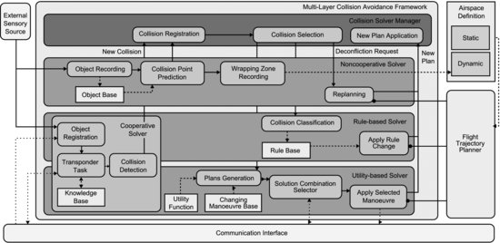
Beside solver modules, there is also the collision solver manager (CSM) – the main controller responsible for the selection of a solver module that will be used for the specific collision. Each solver module has a detection part which is responsible for the detection of a potential future collision. In the case of a cooperative solver module, this detector uses flight intent information which is shared among UAVs locally using data channels. In the case of a non-cooperative solver module, this detector is based on a prediction of the future trajectory based on observations from radar-like data of its surrounding area. Each potential future collision is then registered within CSM. The same collision can be detected by one or several collision solvers.
Depending on the configured priority, CSM assigns each registered collision solver a time slot (considering time to collision) that can be used for its resolution by that solver. Usually, the priorities are configured as preset but they can easily be altered during run-time. At any moment, the CSM has complete information about all reported collisions linked to the time axis. Thus, CSM can perform time-oriented switching among various solvers. Sophisticated switching of collision solvers is inevitable as solvers have different properties. Different solvers provide a different quality of collision-free solution and require a different amount of time to find such solution. Specifically, the negotiation-based solvers may provide a better solution than the non-cooperative solvers due to their coordination, but they usually consume more time as they require negotiation through communication modems. The time to collision is a very important parameter in the multi-layer collision avoidance architecture. The solution of an earlier conflict affects the flight trajectory after that conflict and currently identified collisions after the earlier one can be affected by this resolution. The operation of the collision avoidance framework is permanent, anytime when a solver identifies a new more important collision, the resolution of the currently solved one can be terminated.
9.4.2 Cooperative Collision Avoidance
AgentFly integrates three core cooperative negotiation-based collision avoidance algorithms: (i) rule-based, (ii) iterative peer-to-peer, and (iii) multi-party collision avoidance. All these three methods are decentralized, which means that collisions are solved as localized collision avoidance problems. At the same time, there can also be several (different) algorithms running, resolving various conflicts in different local areas. The local problem is restricted by the defined time horizon. In many of our applications we use a 15-minute time horizon, which correlates with the mid-term collision detection and resolution known from civil air-traffic management. Theoretically, this time horizon can be set to a very large value, which implies that algorithms search for a global collision avoidance solution. All three methods use the same detector part, which is based on sharing of UAVs’ local intentions. These intentions are shared using the subscribe/advertise protocol and are formed as limited parts of their trajectories. UAVs share flight trajectories from the current time moment for the defined time horizon. By acceptation of the subscribe protocol, each UAV makes a commitment that it will provide an update of this limited part of its flight trajectory once its current flight trajectory is modified (e.g. due to other collision or change in its mission tasks) or the already provided part is not sufficient to cover the defined time horizon. This shared information about flight intention is used only to describe the flight trajectory for that time horizon and doesn’t contain any detail about future waypoints and their constraints. So, even though the UAV cooperatively shares its flight intention, it doesn’t disclose its mission to others. Using this mechanism, UAVs build a knowledge-base with local intentions of other UAVs in its surrounding. Every flight intention contains information about the flight execution performance (uncertainty), which is then used along with the separation requirement for the detection of conflicting situations (positions of any two UAVs do not satisfy the required separation distance at any moment in time). This mechanism is robust, as cross conflicts are at least checked by two UAVs.
All three algorithms modify the flight path using the trajectory planner by definition of a replanning task. The modification of the flight trajectory is given by a modification of the waypoint sequence in the request. There can be inserted new, modified existing or removed control waypoints. Please note that collision avoidance cannot alter any waypoint which is defined in the UAV mission defined by the high-level flight controller. There is defined a set of evasion maneuvers which can be applied to the specified location with the specified parameterization. Usually, an evasion maneuver is positioned using the time moment in the flight trajectory and its parameterization defines the strength of the applied maneuver. Seven basic evasion maneuvers are defined: left, right (see Figure 9.7), climb-up, descend-down, fly-faster, fly-slower, and leave-plan-as-it-is evasion maneuvers. The name of each maneuver is given by the modification which it produces. Maneuvers can be applied sequentially at the same place so that this basic set can produce all changes. Each UAV can be configured to use only a subset of these maneuvers or can prioritize some of them. For example, a UAV can be configured to solve conflicts only by horizontal changes (no altitude changes). The leave-plan-as-it-is maneuver is included in the set so that it simplifies all algorithms as they can easily consider the unmodified flight trajectory as one of the options.
Figure 9.7 Application of a right evasion maneuver
9.4.2.1 Rule-Based Collision Avoidance (RBCA)
RBCA is motivated by the visual flight rules defined by the ICAO [28]. Each UAV applies one predefined collision avoidance maneuver means of the following procedure. First, the type of collision between UAVs is determined. The collision type is identified on the basis of the angle between the direction vectors of UAVs in the conflict time projected to the ground plane. Depending on the collision classification and the defined rule for that collision type, each UAV applies the appropriate conflict resolution. Maneuvers are parameterized to use information about the collision and angle so that the solution is fitted to the identified conflict. Application of the resolution maneuver is done by both involved UAVs. This algorithm is very simple and doesn’t require any negotiation during the process of the selection and application of the appropriate collision type solution. The algorithm uses only indirect communication via the updated flight trajectory. Moreover, this algorithm doesn’t use explicitly the cost function including the airplane intention during the collision avoidance search, but the UAVs’ priorities are already included in the flight planner settings which are used during applications, of predefined evasion maneuvers in the rules. Conflicts of more than two UAVs are solved iteratively and the convergence to the stable solution is given by the used rules.
9.4.2.2 Iterative Peer-to-Peer Collision Avoidance (IPPCA)
IPPCA extends the pairwise conflict resolution with negotiation over a set of combinations considering the cost values computed by the involved UAVs. First, the participating UAVs generate a set of new flight trajectories using the configured evasion maneuvers and their lowest parameterization. Only those which do not cause an earlier collision with any known flight trajectory are generated. Each flight trajectory is evaluated and marked with the cost for its application. Then, a generated set of variants are exchanged (including also original unmodified trajectories). During this exchange, the UAV provides only the limited future parts of the trajectories considering the configured time horizon which is the same as used in the conflict detector. Then, the own set of variants and a received set are used to build combinations of trajectories which can be used to resolve the conflict. It can happen that no such combination is found as some variants are removed, because they cause earlier conflicts with others and the rest do not solve the conflict. In such a case, the UAVs extend their sets of new flight trajectories with modifications using higher parameterizations until some combinations are found. The condition removing variants causing earlier collisions is crucial. Without this criterion the algorithm could iterate in an infinite loop and could also generate new conflicts which are so close that they cannot be resolved.
From the set of suitable combinations of flight trajectories, the UAVs select the best combination based on the configured strategy. UAVs can be configured to optimize the global cost (minimize the sum of costs from both UAVs). Or they can be configured as self-interested UAVs. In such a case, they try to reduce the loss caused by their collision. Then, the best possible collision avoidance pair is identified by a variation of the monotonic concession protocol [29] – the protocol for automated agent-to-agent negotiations. Instead of iterative concession on top of the negotiation set, the algorithm can use the extended Zeuthen strategy [30] providing negotiation equilibrium in one step and no agent has an incentive to deviate from the strategy.
9.4.2.3 Multi-party Collision Avoidance (MPCA)
MPCA removes iterations from IPPCA for multi-collision situations – more than two UAVs have mutual future collisions on their flight trajectories. MPCA introduces the multi-party coordinator, who is responsible for the state space expansion and the search for the optimal solution of the multi-collision situation. The multi-party coordinator is an agent whose role is to find a collision-free set of flight trajectories for the whole group of colliding UAVs, considering the limited time horizon. The coordinator keeps information about the group and state space. It chooses which UAV will be invited to the group and requests UAVs to generate modifications of their trajectories. Each state contains one flight trajectory for every UAV in the multi-party group. Initially, the group is constructed from two UAVs which have identified a conflict on their future trajectories. Later, the group is extended with UAVs which have conflicts with them and also which have potential conflicts with any considered flight trajectory in the state space. Similarly to IPPCA, UAVs provide the cost value for the considered collision avoidance maneuver along with its partial future flight trajectory.
The coordinator searches until it finds a state which does not have any collision considering the limited time horizon. Its internal operation can be described as a search loop based on the OPEN list and states. States in OPEN are ordered depending on the used optimization criterion (e.g. the sum of costs, the lowest is the first). In each loop, the coordinator takes the first state and checks if there are some collisions. If there is no collision, trajectories in this state are the solution. If any trajectory has a conflict with other UAV not included in the multi-party group, the coordinator invites this UAV and extends all states with the original flight trajectory of this invited UAV. Then, it selects a pair of UAVs from that state which have the earliest mutual collision and asks them to provide modifications of flight trajectories so that the collision can be eliminated. This step is similar to IPPCA. From the resulting set of options, new children states are generated.
As described above, the participation of UAVs in one multi-party algorithm is determined dynamically by identified conflicts on their trajectories. Thus, two independent multi-party algorithms can run over disjoint sets of UAVs. A UAV already participating in one multi-party run can be invited into other one. In such a case, the UAV decides which one has higher priority and where it will be active based on the earliest collision which is solved by appropriate multi-party runs. The second one is paused until the first one is resolved. Please note that the run-time of the multi-party algorithm is also monitored by the multi-layer collision avoidance framework. The framework can terminate the participation due to lack of time and can select an other solver to resolve the collision.
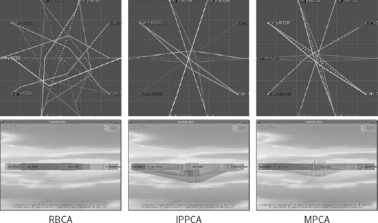
Figure 9.8 presents the different results provided by three presented algorithms in the super-conflict scenario [13] – UAVs are evenly spaced on a circle and each UAV has the destination waypoint on the opposite side of the circle so that the initial flight trajectories go through the center of the circle. RBCA was configured to use only predefined rules not to change altitude. While comparing the quality of solutions, MPCA provides the best solution from these three algorithms. On the other hand, considering the time aspect, MPCA requires the largest amount of time searching for a solution. For detailed results and other experiments, see [27].
Figure 9.8 Results of three cooperative collision avoidance methods in the super-conflict scenario
9.4.3 Non-cooperative Collision Avoidance
AgentFly also integrates the collision avoidance algorithm which doesn’t require a bi-directional communication channel for conflict detection and resolution. In such a case, only radar-like information about objects in its surrounding is used. The method used in AgentFly is based on the dynamic creation of no-flight areas, which are then used by the flight trajectory planner to avoid a potential conflict. Such an approach allows us to combine both cooperative and non-cooperative methods at the same time. The dynamically created no-flight areas are then taken into account when the planner is called by a cooperative solver for application of an evasion maneuver.
Components of the non-cooperative algorithm are displayed in Figure 9.6. The detection part of the algorithm is active permanently. It receives information about positions of objects in the surrounding area. The observation is used to update the algorithm knowledge base. If there is enough history available, the prediction of a potential collision point process is started. The collision point is identified as an intersection of the current UAV’s flight trajectory, and the predicted flight trajectory of the object for which the algorithm receives the radar update. Various prediction methods can be integrated in this component: a simple linear prediction estimating the future object trajectory, including the current velocity, which requires two last positions with time information or a more complex tracking and prediction method based on a longer history, which is also able to track a curve trajectory. The result of the collision point prediction is a set of potential conflict points with a probability of conflict. For many cases, it can happen that there is no such collision point found. Then the previously registered conflict within the collision solver manager is canceled.
In the opposite case, the collision points with higher probability than the configured threshold are wrapped by a dynamic no-flight area. The shape of a dynamic no-flight area is derived from the set of possible collision positions. An example of the shape of a dynamic no-flight area is given in Figure 9.9. The predicted dynamic no-flight area is put to the UAV’s airspace definition database. Such areas are then used by the trajectory planner while it is called by any other component (cooperative collision avoidance algorithm or high-level flight controller). Information about the predicted future collision is also registered within the collision avoidance manager that will decide when the collision will be solved considering the time to collision. Once the non-cooperative solver is asked to solve the collision, the replanning of the current flight trajectory is invoked by calling the flight trajectory planner which keeps the flight trajectory only within the operation airspace excluding all no-flight areas. The modified flight trajectory is then applied for its execution.
Figure 9.9 An example of the shape of a dynamic no-flight area
9.5 Team Coordination
In the presented airplane control architecture, algorithms providing coordination of multiple UAVs are integrated in the high-level flight controller part. The output is formulated as a mission specification which is then passed to the collision avoidance module for its execution. Team coordination is the continuous process. Based on the current status, coordination algorithms can amend the previously provided mission. In AgentFly, there were integrated intelligent algorithms for controlling a group of autonomous UAVs performing information collection in support of tactical missions. The emphasis was on accurate modeling of selected key aspects occurring in real-world information collection tasks, in particular physical constraints on UAV trajectories, limited sensor range, and sensor occlusions occurring in spatially complex environments. Specifically, algorithms are aimed at obtaining and maintaining relevant tactical and operational information up-to-date. Algorithms from this domain primarily address the problems of exploration, surveillance, and tracking. The problem of multi-UAV exploration of an unknown environment is to find safe flight trajectories through the environment, share the information about known regions, and find unexplored regions. The result of the exploration is a spatial map of the initially unknown environment. In contrast, the surveillance is a task providing permanent monitoring of the area. Usually sensors’ coverage of all UAVs is not sufficient to cover the whole area at the same time and UAVs have to periodically visit all places, minimizing the time between visits to the same region. Finally, the tracking task involves such control of UAVs which do not lose the tracked targets from the field of view of their sensors. There are many variants of the tracking tasks based on the different speed of UAVs and tracked targets, as well as the number of UAVs and targets.
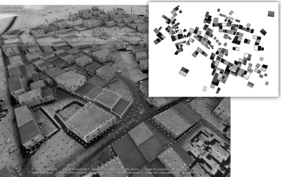
Figure 9.10 shows an example of the scenario which was used for testing of information collection algorithms. In the model, there are more than 300 buildings with different heights and various widths of street in the city. The right top view in Figure 9.10 presents the information known by the group of UAVs once they finished the initial exploration of the unknown area, white buildings are the tallest ones and black ones are the lowest. Initially, UAVs have only planar information about the area taken from a satellite image but they don’t have the full three-dimensional information which is required to perform optimized information collection within that area. Each UAV is equipped with an onboard camera sensor which is oriented downwards. Beside UAVs, there are simulated ground entities – people moving within the city. A simplified behavior was created for people, so that they move intelligently within the city. They react to flying UAVs and other actions. The three-dimensional representation of the urban area plays a crucial role in the scenario. While the UAV is flying over the city, its camera sensor can only see non-occluded areas close to building walls. UAVs have to plan their trajectories carefully, so that they can see to every important place in the city while they perform a persistent surveillance task. The abstraction in the simulation supposes that the image processing software provided with the sensor has the capability to extract high-level information from the obtained data. So, intelligent algorithms which were tested are not working with raw images but with information on a symbolic level. It is supposed that the camera sensor is able to detect edges and identify the height of the building and detect people on the ground. The coverage of one UAV camera sensor is visualized in Figure 9.10.
Figure 9.10 A complex urban scenario used for multi-UAV coordination algorithms
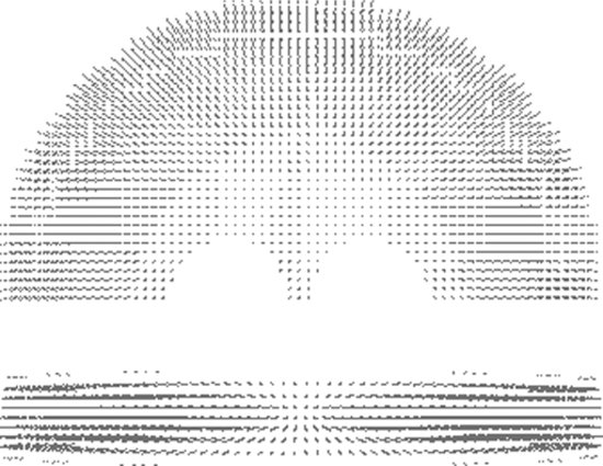
The persistent simulation task can be formulated as an optimization problem, minimizing the objective function. In this case, the objective function is constructed as the sum of information age over the area where the surveillance task should take place. In other words, UAVs try to keep knowledge of any position in the area as recent as possible. The exploration task is just a specific case, where there are some positions in the area with an infinite age, which turns the algorithm to reveal each position by the sensor coverage at least once. During the exploration, UAVs update their unknown information about that area and rebuild a coverage map. A coverage map example is shown in Figure 9.11. The coverage map provides mapping of all interested ground points to air navigation points (waypoints) considering sensor parameters. The multi-UAV simulation task then searches for the flight trajectory patterns (a cyclic trajectory for each UAV) which can be flown at the minimum time so that all interesting points are covered during those cycles. The intelligent algorithm for persistent surveillance searches for such trajectories and allocates them to available UAVs. The situation becomes more complex when several surveillance areas are defined and airplanes have to be assigned to particular areas or have to cycle between them in order to keep minimized the objective function during the time. Detailed results from the information collection algorithms implemented in AgentFly can be found in [31].
Figure 9.11 A coverage map in the urban area
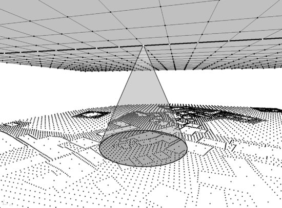
Figure 9.12 The tracking task of a ground entity
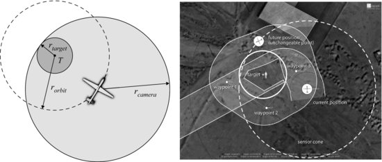
The tracking task requires that a ground target is covered by the UAV’s sensor for the whole time. Thus, it should provide an uninterrupted stream of image data about a designated target. Tracking is a challenging task because of the lack of knowledge of a target’s future plans and the motion constraints of the UAV. In AgentFly, a circular pattern navigation algorithm is integrated for one UAV which is tracking one target, see Figure 9.12. A virtual circle is constructed above the tracked object – the radius of the circle is derived from motion constraints of the UAV as small as possible to keep the UAV close to the tracked object. The UAV tries to stay on this circular trajectory as this is the best trajectory to keep the tracked object covered by its camera sensor. While the tracked object is moving (in our case it is moving slower than the maximum flight speed of the UAV), the virtual circle moves with it. As described in Section 9.2, the algorithm has to provide a mission for the UAV in the form of a sequence of waypoints. The UAV, considering the current position and the optimal virtual circle, computes positions for waypoints based on the tangent projection from the current position. Then it prepares the next waypoints around the circle. The algorithm is invoked once it gets updated positions of the tracked object. In such a case, the tracking algorithm adjusts the position of computed waypoints if necessary. The algorithm becomes more complex when one UAV is tracking a cluster of ground targets at the same time. In this case, the UAV uses a general orbit trajectory instead of a virtual circle.
Figure 9.13 Command and control panel in AgentFly
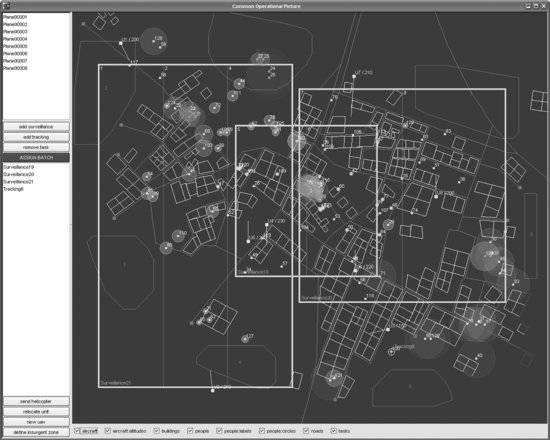
Figure 9.13 provides a view of the interface for the interaction with the system. This interface is provided by an agent which implements the hybrid command and control system for mixed information collection tasks. Through this agent, a human operator can specify information collection tasks for the whole group of UAVs and inspect the resulting operation. The agent automatically collects knowledge about the area and presents it to the operator. Tasks are not defined for particular UAVs but are specified as goals for the whole group. Thus, a multi-agent allocation algorithm is integrated for the optimal allocation of concurrent information collection tasks in the group. There is no centralized element in this system. The command and control system adopts a robust solution which implies that UAVs synchronize and merge partial information together anytime they can communicate together. If any UAV is lost, the group loses only information which was not synchronized within the group and information collection tasks are reorganized so that the remaining UAVs fulfill the requested tasks considering the configured optimization objective function. Similarly, when a new UAV is added to the group, it gets synchronized while it establishes communication with any other UAV in the group. The command and control agent needs a connection only with one UAV in the group.
9.6 Scalable Simulation
Thanks to the agent-based approach used, AgentFly can provide a simulation environment to model and study complex systems with a large number of situated entities, high complexity of their reasoning and interactions. For such a complex system, it is not possible to run the whole simulation system hosted on a single computer. AgentFly provides an effective distribution schema which splits the load over heterogenous computers connected through a fast network infrastructure. Within the AgentFly simulation environment, not only can UAVs or civilian airplanes be simulated, but any type of situated entity. By situated entity we mean an entity embedded in a synthetic model of a three-dimensional physical space. AgentFly provides high-fidelity (accurate simulation with respect to the defined physics, not using level of details), scalable (in terms of the number of simulated entities and the virtual world dimension), and fast (produce results for a simulated scenario in the minimum possible time) simulation platform. The development of such functionality has been motivated initially by the need to simulate full civilian air-traffic in the national airspace of the United States, with great level of detail. Further, the same feature has been used to validate intelligent algorithms for UAVs which operate in very complex environments – beside a high number of UAVs there are simulated ground vehicles and running models of people that play a crucial role in the scenario.
The AgentFly simulation supports both passive (their behavior is only defined by their physics) and autonomous (pro-active, goal-oriented actors) situated entities operating and interacting in a realistically modeled large-scale virtual world. Entities could be dynamically introduced or removed during the simulation run-time based on the evaluation scenario needs. Each situated entity carries a state – the component which can be either observable (public) or hidden (private, internal). The fundamental component of the entity’s observable state is its position and orientation in the virtual world (e.g. the position of the UAV). The evolution of the entity’s state is governed by the defined entity’s physics, e.g. the entity's movement is driven by its motion dynamics, typically defined by a set of differential equations which can also refer to the entity’s hidden state components. Physics can be divided into intra-entity and inter-entity parts. The intra-entity physics capture those aspects of physical dynamics that can be fully ascribed to a single entity. Although the equations of the intra-entity physics can refer to any state in the simulated world (e.g. weather condition), they only govern the states carried by its respective entity. In contrast, the inter-entity physics captures the dynamics that affects multiple entities simultaneously and cannot be fully decomposed between them (e.g. the effects of a physical collision of two UAVs). Beside physical interactions, autonomous entities can also interact via communication and use sensors to perceive their surrounding virtual environment. Communication between entities can be restricted by the inter-entity physics simulating a required communication medium (e.g. wireless network). Similarly, each sensor has its capabilities defined, which may restrict the observable state it can perceive only to a defined subset, typically based on the distance from the sensor’s location (e.g. radar, onboard camera).
Each situated entity (e.g. UAV) in AgentFly is divided into up to three sub-components: (i) body, (ii) reactive control, and (iii) deliberative control. The body encapsulates the entity’s intra-physics, which governs the evolution of its state as a function of other, possibly external states (e.g. UAV flight dynamics given by the motion model used affected by the current atmospheric condition). The reactive control component contains a real-time loop-back control for the entity, affecting its states based on the observation of other states (e.g. the flight executor component integrating the autopilot function for the UAV). The deliberative control component contains complex intelligent algorithms employing planning, sensing observations, and communication with others (the flight trajectory planner, collision avoidance framework, and high-level flight controller in the UAV control architecture). The outputs of deliberative control typically feed back into the entity’s reactive control module and provide a new control for the entity (the update of the current flight trajectory in the UAV). The body and reactive control components are similar in their loop-back approach and are collectively referred to as the entity’s state updater.
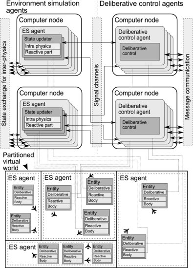
As described in Section 9.1, AgentFly is implemented as the multi-agent system with environmental simulation agents and UAV agents which contains intelligent deliberative algorithms. Figure 9.14 presents the decomposition of components of each UAV into software agents. Thanks to the Aglobe multi-agent framework used, each computer node can host one or several agents and an efficient communication infrastructure is available. Within the simulation architecture, the deliberative controller and state updater of each entity are decoupled and integrated within different agents. The respective pair of state updater and deliberative controller is connected by a signal channel through which sensing perceptions (one way) and control commands to the reactive control (the other way) are transmitted.
Figure 9.14 The distributed simulation approach in AgentFly
AgentFly employs a time-stepped simulation approach – the virtual simulation time driving the dynamic processes of the simulation is incremented uniformly by a constant time step in each simulation cycle. All physics and reactive parts of all entities have to be evaluated synchronously in order to provide consistent evolution of the virtual world. Synchronous evaluation means that states are updated once all physics is computed based on the previous state. The virtual time steps and thus state updates can be applied regularly with respect to the external wall clock time or in a fast-as-possible manner. The first mode has to be used when AgentFly is running as a hybrid simulation (the part of the scenario is simulated, some entities are represented by real hardware). Within the simulation mode, the fast-as-possible mode is used in order to get simulation results in the shortest possible time – the next step (simulation cycle) is initiated immediately after the previous one has been completed.
Both environment simulation and deliberative control agents are distributed among multiple computer nodes during the simulation. The whole virtual simulation world is spatially divided into a number of partitions. The partitions are mutually disjoint except for small overlapping areas around partitions’ boundaries. Each partition has a uniquely assigned environment simulation agent (ES agent) responsible for updating states (e.g. applying relevant differential equations) corresponding to all entities located within its assigned partition. The number of ES agents running on one computer node is limited by the number of processing cores at that node. The application of physics may require exchange of state information between multiple partitions, in case affected entities are not located within the same partition. In contrast with the state updaters, entities’ deliberative control parts are deployed to computer nodes irrespective of the partitions and corresponding entity’s position in the virtual world. The described world partitioning implies that whenever the location of an entity changes so that the entity moves to a new partition, the entity’s state updater needs to be migrated to the respective ES agent. The signal channel between the entity’s control and its deliberative control modules is transparently reconnected and it is guaranteed that no signal transmission is lost during the migration. The small overlapping areas around partition boundaries are introduced to suppress oscillatory migration of state updaters between neighboring ES agents in case the corresponding entity is moving very close along a partition border.
In order to provide maximum performance throughout the whole simulation, the proposed architecture implements load-balancing approaches applied to both environment simulation agents and deliberative control agents. The virtual world decomposition to partitions is not fixed during the simulation but is dynamically updated depending on the load of computer nodes hosting environment simulation agents. Based on the time required for processing the simulation cycle, the virtual world is repartitioned so that the number of entities belonging to partitions is proportional to the measured times. The ES agent that is faster will be assigned a larger area with more entities and vice versa. Repartitioning is not performed during each simulation cycle but only if the difference in simulation cycle computation by various ES agents exceeds a predefined threshold. It is also triggered whenever a new computer node is allocated for simulation. Similarly, the deliberative components are split among computer nodes based on the load of those computers.
Figure 9.15 presents the results, studying the dependency of the simulation performance on the number of computer nodes. In this experiment, the same number of UAVs was simulated in all configurations. A 1-day scenario was simulated with more than 20,000 UAVs performing various flight operations within that day. There were about 2000 flying UAVs at the same moment in time. The number of simultaneous flying UAVs varied slightly in the scenario.
Figure 9.15 The result of varying number of computation nodes available for the simulation
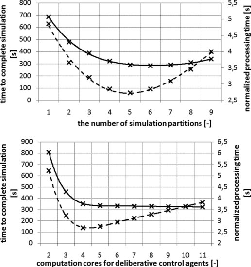
The left chart in Figure 9.15 presents the dependency of the time to complete the whole scenario on the number of computer nodes available for the environment simulation (thus the number of partitions and ES agents). UAV agents are running in every configuration on the same number of computers. We can observe that there are three utilization regions: (i) over-loaded, (ii) optimally loaded, and (ii) under-loaded. In the left part (1, 2, and 3 partitions), the normalized processing time1 is significantly decreased with more partitions (few ES agents are over-loaded by computing inter-physics). For the mid-part (4 and 5 partitions), the normalized processing time stagnates, which is caused by rising demands for partition-to-partition coordinations. Adding even more computation resources (and thus more partitions) results in a decreasing normalized processing time, the simulation is under-loaded – the overhead for synchronization dominates the parallelized processing. The right chart in Figure 9.15 studies varying computational resources available for deliberative control agents (UAV agents). In this case, the fixed number of partitions was used. Similarly to the previous case, in the left part there is a significant speed-up given by parallelization of execution of heavy-weight agents and for less computational power all CPUs are over-loaded and the simulation is slower. For increasing resources, the time to complete simulation is almost unchanging. In this case, the overall simulation bottle neck is not in the efficiency of UAV agents, but in the limit of the environment simulation. The increasing resources (6, 7, and more) are wasted and thus the normalized processing time is increased due to an increase in the processing time. In contrast to the left chart, addition of more resources for deliberative controller agents doesn’t slow down the whole simulation (does not cause coordination overhead for the simulation).
9.7 Deployment to Fixed-Wing UAV
AgentFly is deployed to various UAV platforms including a quad-rotor helicopter. This chapter presents the deployment to the fixed-wing airplane called Procerus UAV. Our Procerus UAV is shown in Figure 9.16. We use this small UAV as we can easily perform experiments and we are not restricted by any regulation. Once AgentFly is able to provide all intelligent algorithms for a small UAV, it can be used successfully for the control of any larger and more equipped one. UAV is based on the Unicorn airframe from EPP foam with 72” wingspan. It is a fully autonomous UAV which has installed four Li-pol batteries, Kestrel autopilot board, data communication modem with antenna, GPS unit, electric motor with necessary power regulator and currency sensor, servos for ailerons, motorized gimbal camera (installed on the bottom side), video transmitter with antenna, and AgentFly CPU board. The weight of the fully loaded UAV platform is about 3 kg. Depending on the number of take-offs, climbs, and usage of the onboard camera system, it can fly up to 60 minutes with a speed from 40 to 65 mph. Now, we primarily use these UAVs for experimentation with described autonomous algorithms for sense and avoid. Thus, the camera system is not connected to the onboard processer but the video is broadcasted to the ground station, see Figure 9.17. The gimbal camera system is electrically retractable (which is usually done before landing), and the operator can control pan, tilt, and zoom of the camera. Even though the communication modem is able to keep connection for several miles the, UAV is able to fly autonomously without connection to the ground station as the AgentFly system is running onboard.
Figure 9.16 Procerus UAV – the fixed-wing airplane
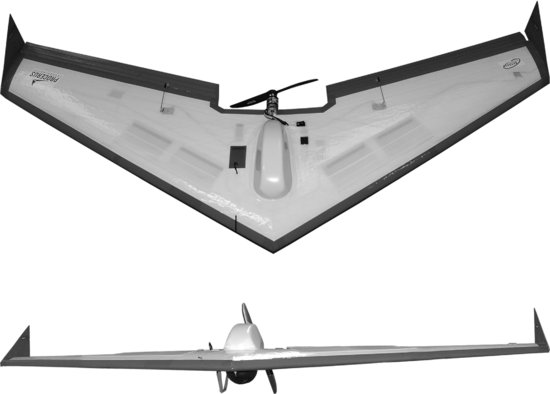
Figure 9.17 The screenshot from a camera feed transmitted to the ground station
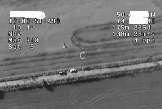
Figure 9.18 Assisted autonomous take-off (left) and landing (right)
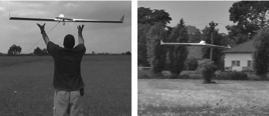
The autopilot board has integrated three-axis gyros, accelerometers, magneto-meter, absolute and differential pressure sensors for altitude/airspeed, and there are also integrated temperature sensors for compensation of sensors’ drifts in changing temperature. The autopilot uses the GPS unit for its navigation and also estimation of the wind speed and heading, which helps it achieve better control. The AgentFly CPU board is connected through a serial link with the autopilot so that it can read the current flight performance including position data from GPS and provide a control back to the autopilot. The AgentFly CPU board is the Gumstix computer module with ARM Cortex-A8 CPU (RISC architecture) running AgentFly in JAVA. We use the same implementation for the UAV control as is used in the simulation mode. There are only changed interfaces so that sensors, communication channel, and flight executor are mapped to the appropriate hardware. The autopilot is able to control the UAV and navigate it through the provided waypoints. It also supports assisted autonomous take-off (the UAV is thrown from the hand or launched from a starting gun; its autonomous take-off procedure is invoked when the UAV reaches the appropriate speed threshold) and autonomous landing in the defined area, see Figure 9.18. The autopilot is not able to track the flight trajectory intention as described in Section 9.2. Thus, the part of the functionality from the flight executor is running on the AgentFly CPU board. Based on the UAV’s parameters, the flight executor converts the flight trajectory intention into a sequence of low-level navigation waypoints which are passed to the autopilot board through the serial connection. These navigation waypoints are selected so that the UAV platform follows the requested trajectory as precisely as possible. On the other hand, the flight executor contains a monitoring module which permanently processes the flight status (including the GPS position and wind estimation) and checks if the flight is executed within the defined tolerance. The monitor module invokes replanning and adjusting the flight performance prediction. For some future version, a module can be integrated that will automatically adjust preconfigured parameters of the UAV model used by the flight trajectory planner. This will minimize the number of replannings when preconfigured parameters don’t fit well for the current conditions.
Agents running on the AgentFly CPU board can communicate with other UAVs and also with the ground system through the data communication modem which is connected to the autopilot. Now, we haven’t any source for radar-like information about objects in the UAV’s surrounding area. We are only working with the cooperative collision avoidance algorithms which utilize negotiation-based conflict identification as described in Section 9.4. All UAVs, both real and simulated, are flying in the same global coordination system.
Acknowledgments
The AgentFly system has been sponsored by the Czech Ministry of Education grant number 6840770038 and by the Federal Aviation Administration (FAA) under project numbers DTFACT-08-C-00033 and DTFACT-10-A-0003. Scalable simulation and trajectory planning have been partially supported by the CTU internal grant number SGS10/191/OHK3/2T/13. The underlying AgentFly system and autonomous collision avoidance methods have been supported by the Air Force Office of Scientific Research, Air Force Material Command, USAF, under grant number FA8655-06-1-3073. Deployment of AgentFly to a fixed-wing UAV has been supported by the Czech Ministry of Defence grant OVCVUT2010001. The views and conclusions contained herein are those of the authors and should not be interpreted as representing the official policies or endorsements, either expressed or implied, of the Federal Aviation Administration, the Air Force Office of Scientific Research, or the US Government.
References
1. M. Šišlák, M. Rehák, M. P![]() chou
chou![]() ek, M. Rollo, and D. Pavlí
ek, M. Rollo, and D. Pavlí![]() ek. AGLOBE: Agent development platform with inaccessibility and mobility support. In R. Unland, M. Klusch, and M. Calisti (eds), Software Agent-Based Applications, Platforms and Development Kits, pp. 21–46, Berlin Birkhauser Verlag, 2005.
ek. AGLOBE: Agent development platform with inaccessibility and mobility support. In R. Unland, M. Klusch, and M. Calisti (eds), Software Agent-Based Applications, Platforms and Development Kits, pp. 21–46, Berlin Birkhauser Verlag, 2005.
2. M. Wooldridge. An Introduction to MultiAgent Systems. John Wiley & Sons Inc., 2002.
3. P. Santi. Topology Control in Wireless Ad-hoc and Sensor Networks. John Wiley & Sons Inc., 2005.
4. R. Schulz, D. Shaner, and Y. Zhao. Free-flight concept. In Proceedings of the AIAA Guidance, Navigation and Control Conference, pp. 889–903, New Orleans, LA, 1997.
5. National Research Council Panel on Human Factors in Air Traffic Control Automation. The future of air traffic control: Human factors and automation. National Academy Press, 1998.
6. G.J. Pappas, C. Tomlin, and S. Sastry. Conflict resolution in multi-agent hybrid systems. In Proceedings of the IEEE Conference on Decision and Control, Vol. 2, pp. 1184–1189, December 1996.
7. K.D. Bilimoria. A geometric optimization approach to aircraft conflict resolution. In Proceedings of the AIAA Guidance, Navigation, and Control Conference, Denver, August 2000.
8. J. Gross, R. Rajvanshi, and K. Subbarao. Aircraft conflict detection and resolution using mixed geometric and collision cone approaches. In Proceedings of the AIAA Guidance, Navigation, and Control Conference, Rhode Island, 2004.
9. A.C. Manolis and S.G. Kodaxakis. Automatic commercial aircraft-collision avoidance in free flight: The three-dimensional problem. IEEE Transactions on Intelligent Transportation Systems, 7(2):242–249, June 2006.
10. J. Hu, M. Prandini, and S. Sastry. Optimal maneuver for multiple aircraft conflict resolution: A braid point of view. In Proceedings of the 39th IEEE Conference on Decision and Control, Vol. 4, pp. 4164–4169, 2000.
11. M. Prandini, J. Hu, J. Lygeros, and S. Sastry. A probabilistic approach to aircraft conflict detection. IEEE Transactions on Intelligent Transportation Systems, 1(4):199–220, December 2000.
12. A. Bicchi and L. Pallottino. On optimal cooperative conflict resolution for air traffic management systems. IEEE Transactions on Intelligent Transportations Systems, 1(4):221–232, December 2000.
13. L. Pallottino, E.M. Feron, and A. Bicchi. Conflict resolution problems for air traffic management systems solved with mixed integer programming. IEEE Transactions on Intelligent Transportation Systems, 3(1):3–11, March 2002.
14. Federal Aviation Administration. Aeronautical Information Manual. Federal Aviation Administration, US Department of Transportation, 2008.
15. C.R. Spitzer. Avionics: Elements, Software and Functions. CRC, 2006.
16. P. Hart, N. Nilsson, and B. Raphael. A formal basis for the heuristic determination of minimum cost paths. IEEE Transactions on Systems Science and Cybernetics, (2):100–107, 1968.
17. D. Šišlák, P. Volf, and M. P![]() chou
chou![]() ek. Flight trajectory path planning. In Proceedings of the 19th International Conference on Automated Planning & Scheduling (ICAPS), pp. 76–83, Menlo Park, CA. AAAI Press, 2009.
ek. Flight trajectory path planning. In Proceedings of the 19th International Conference on Automated Planning & Scheduling (ICAPS), pp. 76–83, Menlo Park, CA. AAAI Press, 2009.
18. P. Yap. Grid-based path-finding. In Proceedings of the Canadian Conference on Artificial Intelligence, pp. 44–55, 2002.
19. D. Šišlák. Autonomous Collision Avoidance in Air-Traffic Domain. PhD thesis, Czech Technical University, Prague, February 2010.
20. A. Nash, K. Daniel, S. Koenig, and A. Felner. Theta*: Any-angle path planning on grids. In Proceedings of the AAAI Conference on Artificial Intelligence (AAAI), pp. 1177–1183, 2007.
21. S.M. LaValle and J.J. Kuffner. Rapidly exploring random trees: Progress and prospects. In B.R. Donald, K.M. Lynch, and D. Rus (eds), Algorithmic and Computational Robitics: New Directions, pp. 293–308, A.K. Peters, Wellesley, MA, 2001
22. A. Yershova, L. Jaillet, T. Siméon, and S.M. LaValle. Dynamic-Domain RRTs: Efficient exploration by controlling the sampling domain. In Proceedings of the IEEE International Conference on Robotics and Automation, pp. 3867–3872, 2005.
23. A. Botea, M. Müller, and J. Schaeffer. Near optimal hierarchical path-finding. Journal of Game Development, 1(1):7–28, 2004.
24. D. Ferguson and A. Stentz. Using interpolation to improve path planning: The field D* algorithm. Journal of Field Robotics, 23(1):79–101, 2006.
25. D. Šišlák, P. Volf, and M. P![]() chou
chou![]() ek. Accelerated A* trajectory planning: Grid-based path planning comparison. In Proceedings of the 19th International Conference on Automated Planning & Scheduling (ICAPS), pp. 74–81, Menlo Park, CA. AAAI Press, 2009.
ek. Accelerated A* trajectory planning: Grid-based path planning comparison. In Proceedings of the 19th International Conference on Automated Planning & Scheduling (ICAPS), pp. 74–81, Menlo Park, CA. AAAI Press, 2009.
26. Š. Kop![]() iva, D. Šišlák, D. Pavlí
iva, D. Šišlák, D. Pavlí![]() ek, and M. P
ek, and M. P![]() chou
chou![]() ek. Iterative accelerated A* path planning. In Proceedings of 49th IEEE Conference on Decision and Control, December 2010.
ek. Iterative accelerated A* path planning. In Proceedings of 49th IEEE Conference on Decision and Control, December 2010.
27. D. Šišlák, P. Volf, and M. P![]() chou
chou![]() ek. Agent-based cooperative decentralized airplane collision avoidance. IEEE Transactions on Intelligent Transportation Systems, 12(1):36–46, March 2011.
ek. Agent-based cooperative decentralized airplane collision avoidance. IEEE Transactions on Intelligent Transportation Systems, 12(1):36–46, March 2011.
28. M.S. Nolan. Fundamentals of Air Traffic Control, 4th edn. Thomson Brooks/Cole, Belmont, CA, 2004.
29. G. Zlotkin and J.S. Rosenschein. Negotiation and task sharing among autonomous agents in cooperative domains. In Proceedings of the 11th International Joint Conference on Artificial Intelligence, pp. 912–917, San Mateo, CA. Morgan Kaufmann, 1989.
30. F.L.B. Zeuthen. Problems of Monopoly and Economic Warfare. Routledge and Sons, 1930.
31. E. Semsch, M. Jakob, D. Pavlí![]() ek, M. P
ek, M. P![]() chou
chou![]() ek, and D. Šišlák. Autonomous UAV surveillance in complex urban environments. In C. McGann, D.E. Smith, M. Likhachev, and B. Marthi (eds), Proceedings of ICAPS 2009 Workshop on Bridging the Gap Between Task and Motion Planning, pp. 63–70, Greece, September 2009.
ek, and D. Šišlák. Autonomous UAV surveillance in complex urban environments. In C. McGann, D.E. Smith, M. Likhachev, and B. Marthi (eds), Proceedings of ICAPS 2009 Workshop on Bridging the Gap Between Task and Motion Planning, pp. 63–70, Greece, September 2009.
1. The normalized processing time expresses the computational real time (wall clock) per one UAV in the simulation.