
7
UAS Conflict Detection and Resolution Using Differential Geometry Concepts
7.1 Introduction
The large-scale military application of unmanned aircraft systems (UAS) is generating operating experience and technologies that will enable the next phases of utilisation. An important driver for future growth of UAS is in the civil commercial sector, which could emerge as the largest user in due course. The employment of UAS for military operations and civil commercial use remains restricted to operations mostly in segregated airspace. Integrating UAS into non-segregated airspace is the key enabler for dramatic development of many new and innovative applications. Therefore, it is likely that UAS integration into non-segregated airspace will be enabled as demand from operators materialises. Collision detection and resolution (CD&R) – i.e., sense and avoid – would be a major step towards allowing UAS integration into non-segregated airspace.
The CD&R algorithm has been considered an important problem ever since aircraft were developed. Moreover, there have been numerous studies and implementations of it. Thus far most CD&R algorithms have been performed by air traffic control (ATC) from the ground station [1]. However, the ground station-based air traffic control would have limited coverage capability to cope with dramatic increases in air traffic [2]. Free flight including an autonomous CD&R algorithm, operated by an onboard computer, can reduce the burden on the ground station-based air traffic control [3]. This has become a possible option to consider due to the development of onboard computer and sensor technology.
A number of different approaches have been applied to the CD&R problem [4]. Collision avoidance using a potential function has been investigated since the first study by Khatib [5]. In essence, this method uses an artificial potential field which governs UAS kinematics, but cannot always guarantee that the relative distance is greater than a minimum safe separation distance due to the difficulty of predicting the minimum relative distance. Intelligent control has also been introduced as the new control theory [6] and implemented in the CD&R algorithm [7, 8]. A CD&R algorithm based on the hybrid system has been studied at Stanford University and UC Berkeley [2,9]. In this research, cooperating vehicles resolve the conflict by specific manoeuvres such as level flight, coordinate turn, or both under the assumption that all information is fully communicated. There have also been studies of a hybrid CD&R algorithm using the Hamilton–Jacobi–Bellan equation and hybrid collision avoidance with ground obstacles using radar [10, 11].
Since traffic collision alerting system (TCAS) equipment with an onboard pilot has been used in civil aviation, a number of studies and flight tests on TCAS-like CD&R for UAS have been investigated over the past decades [12--14]. TCAS provides resolution advisories with vertical manoeuvre command, and these advisories are based on various experiences and a great database, not analytical verification [2]. However, it is possible to guarantee the high reliability of TCAS by statistical analysis. The accident rate is lower than 1% per year with respect to 50 possible accidents in the case of aircraft not equipped with TCAS [13]. UAS Battlelab has studied to develop TCAS on high-performance UAS such as Global Hawk in non-military airspace. Cho et al. [13] proposed the TCAS algorithm on UAS by converting TCAS vertical commands into UAS autopilot input and analysed its performance by numerical examples. Lincoln Laboratory, MIT published the result in 2004 [15]. Furthermore, the Environmental Research Aircraft and Sensor (ERAST) has investigated collision avoidance systems with TCAS-II and radar by experimentation. As a new concept of collision avoidance, air vehicles communicate their information using ADS-B. The Swedish Civil Aviation Administration (SCAA) performed flight tests for a medium-altitude long-endurance (MALE) UAS – the Eagle – produced by European Aeronautic Defense and Space Company (EADS) and Israel Aircraft Industries (IAI) to make a landing from one civil airport to another outside Kiruna with the concept of IFR (instrument flight rules) using a remote pilot in 2002 [16]. The Eagle UAS was equipped with a standard Garmin ATC transponder as well as a ADS-B VDLm transponder [4]. However, it is difficult to analytically verify these approaches and consider limitations caused by physical and operational constraints such as a relatively low decent/climb or turning rate.
The main issue with the CD&R is whether the algorithm can guarantee collision avoidance by strict verification, because the CD&R algorithm is directly related to the safety of the aerial vehicle. In this study, the cases for both single and multiple conflicts are considered for a single UAS. Two CD&R algorithms are proposed using the differential geometry concepts: one controls the heading angle alone and the other controls it with the ground speed. The proposed algorithms also use the principles of airborne collision avoidance systems [17, chapter 14] conforming to TCAS. Moreover, their stability and feasibility are examined using rigorous mathematical analysis, not using the statistical analysis as in the TCAS algorithm. In order to design the algorithms, we first introduce the definitions of the conflict, conflict detection and conflict resolution by using the same concepts as in [18, 19], such as the closest approach distance (CAD) and the time to closest point of approach (TCPA). Then, conflict resolution guidance will be proposed after deriving the geometric requirements to detect and resolve the conflict. The proposed algorithms are modified from previous research undertaken by the authors and presented in [20, 21].
The study limits the analysis to non-cooperating UAS and intruders, which is denoted as aircraft in this chapter, as this is more challenging in the CD&R problem. It is also assumed that:
- Vehicle dynamics are represented by point mass in Cartesian coordinates on
 .
. - Aircraft are non-manoeuvring for collision avoidance.
- UAS can obtain the deterministic position and velocity vectors of aircraft by using sensors, a communication system or estimator.
This implies that UAS predict the trajectories and future state information using the current position and velocity vector and their linear projections. Note that these assumptions are for ease of analysis and are not a restriction of the approach.
7.2 Differential Geometry Kinematics
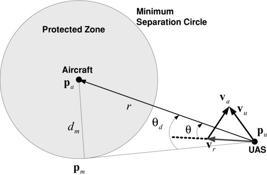
Consider the scenario shown in Figure 7.1, where a UAS is following a prescribed path and an aerial vehicle is crossing the path with the possibility of interception.
Figure 7.1 Guidance geometry (modified from [21])
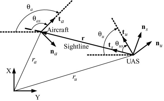
The UAS senses the aircraft and establishes a sightline between it and the aircraft. Assuming the velocity of the aircraft is known (usually using a motion estimator), the motion geometry can be defined. Several axis sets can be defined. A tangent and normal basis vector set ![]() defines the sightline, with
defines the sightline, with ![]() defining the UAS and
defining the UAS and ![]() defining the aircraft. From Figure 7.1, the sightline range vector is given by
defining the aircraft. From Figure 7.1, the sightline range vector is given by
If the assumption is made that both the UAS and the aircraft velocity is constant, then the differential of equation (7.1) yields
This equation represents the components of the aircraft velocity relative to the UAS. Components of the relative velocity along and normal to the sightline are given by projection onto the basis vectors ![]() and
and ![]() . Hence:
. Hence:
The UAS-to-aircraft relative acceleration is given by differentiating equation (7.2) and noting
(7.4) ![]()
to give
(7.5) ![]()
The Serret–Frenet equations for the UAS and the aircraft can be rewritten in terms of a constant velocity trajectory in the form
(7.6) ![]()
where ![]() is the curvature of the trajectory and
is the curvature of the trajectory and ![]() is the instantaneous rotation rate of the Serret–Frenet frame about the bi-normal vector
is the instantaneous rotation rate of the Serret–Frenet frame about the bi-normal vector ![]() . The normal vector
. The normal vector ![]() is a unit vector that defines the direction of the curvature of the trajectory (cf. Figure 7.1) and the bi-normal vector
is a unit vector that defines the direction of the curvature of the trajectory (cf. Figure 7.1) and the bi-normal vector ![]() is orthonormal to
is orthonormal to ![]() and
and ![]() , forming a right-handed triplet (
, forming a right-handed triplet (![]() ,
, ![]() ,
, ![]() ). Hence:
). Hence:
(7.7) ![]()
Components along and normal to the sightline can be determined by projection onto the basis vectors ![]() and
and ![]() , to give
, to give
Equation (7.8) describes the acceleration kinematics of the engagement and equation (7.3) describes the velocity kinematics.
7.3 Conflict Detection
7.3.1 Collision Kinematics
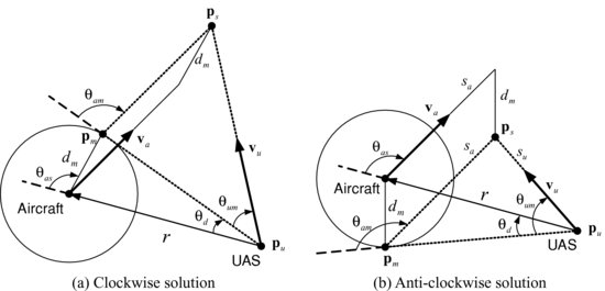
In order to develop conflict detection and resolution algorithms, the collision conditions are first investigated. The geometry and matching conditions of a non-manoeuvring aircraft with a direct, straight line UAS collision trajectory are shown in Figure 7.2(a, b).
Figure 7.2 Collision geometry (modified from [21])
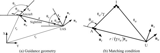
Note that the intercept triangle AIU does not change shape, but shrinks as the UAS and aircraft move along their respective straight-line trajectories. The UAS-to-sightline angle ![]() and the aircraft-to-sightline angle
and the aircraft-to-sightline angle ![]() remain constant over the whole engagement. As shown in Figure 7.3, a useful interpretation of this condition can be visualised if the relative velocity of the UAS with respect to the aircraft is considered.
remain constant over the whole engagement. As shown in Figure 7.3, a useful interpretation of this condition can be visualised if the relative velocity of the UAS with respect to the aircraft is considered.
Figure 7.3 Relative velocity for collision (from [21])
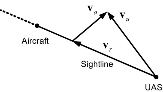
In the figure, the relative velocity of the UAS with respect to the aircraft, ![]() , is denoted
, is denoted
The collision condition is shown to be such that the relative velocity vector should lie along the sightline. This ensures that the sightline will not change direction, but only change in length and so the geometry remains the same over time.
From the intercept triangle in Figure 7.2(b), we have
(7.10) ![]()
Noting that
(7.11) ![]()
gives
Equation (7.12) can be visualised as a vector addition, and is shown in Figure 7.2(b). It is in a non-dimensional form and will thus represent the solution for all ranges between the UAS and the aircraft. The ratio ![]() is fixed for the whole solution and thus as the range r decreases, so will the aircraft arc length
is fixed for the whole solution and thus as the range r decreases, so will the aircraft arc length ![]() . Given the geometry of the aircraft basis vector
. Given the geometry of the aircraft basis vector ![]() and the range basis vector
and the range basis vector ![]() , the direction of the UAS basis vector
, the direction of the UAS basis vector ![]() is fixed. In equation (7.12), the ratio
is fixed. In equation (7.12), the ratio ![]() can be obtained by applying the cosine rule in Figure 7.2(b). From the figure, we have
can be obtained by applying the cosine rule in Figure 7.2(b). From the figure, we have
This quadratic in ![]() can be solved explicitly, to give
can be solved explicitly, to give
(7.14) ![]()
Given that both ![]() and
and ![]() , the solution will exist for any
, the solution will exist for any ![]() such that
such that
(7.15) ![]()
The collision direction can easily be determined from Figure 7.3. This is because, when the collision geometry meets the kinematic condition in equation (7.13) and hence the geometric condition in equation (7.12), the geometry is invariant and the relative velocity ![]() defined in equation (7.9) and shown in Figure 7.3 defines the approach direction.
defined in equation (7.9) and shown in Figure 7.3 defines the approach direction.
7.3.2 Collision Detection
Based on the concept of collision geometry, an algorithm detecting the danger of collision is established. If the distance between the UAS and the aircraft is or will be smaller than the minimum separation of ![]() within a specific time, it is said that there is a conflict in which the UAS and the aircraft experience a loss of minimum separation. Although this does not in itself mean that there exists a danger of collision, it represents the level of danger. In this study, the minimum separation, the CAD and TCPA are used to detect the conflict between the UAS and the aircraft.
within a specific time, it is said that there is a conflict in which the UAS and the aircraft experience a loss of minimum separation. Although this does not in itself mean that there exists a danger of collision, it represents the level of danger. In this study, the minimum separation, the CAD and TCPA are used to detect the conflict between the UAS and the aircraft.
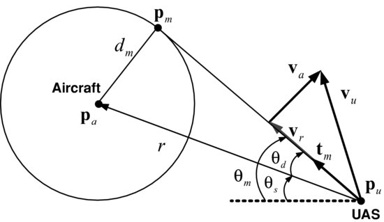
The sightline geometry is shown in Figure 7.4.
Figure 7.4 Sightline geometry for single UAS and aircraft
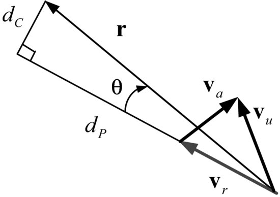
For a non-manoeuvring aircraft, the CAD ![]() can be derived by projecting the relative position vector along the sightline:
can be derived by projecting the relative position vector along the sightline:
(7.16) ![]()
where ![]() denotes the angle from the sightline to the relative velocity vector. TCPA
denotes the angle from the sightline to the relative velocity vector. TCPA ![]() is, thus, determined as
is, thus, determined as
(7.17) ![]()
where ![]() denotes the relative distance travelled to the CPA in the form
denotes the relative distance travelled to the CPA in the form
(7.18) ![]()
From the CAD and TCPA, the conflict is defined as: the UAS and aircraft are said to be in conflict if the CAD is strictly smaller than the minimum separation of ![]() and the TCPA is in the future but before the look-ahead time T, i.e.
and the TCPA is in the future but before the look-ahead time T, i.e.
(7.19) ![]()
Figure 7.5 shows a scenario in which a conflict exists between a UAS and an aircraft.
Figure 7.5 CD&R geometry (modified from [20])
In the figure, the protected zone of the aircraft is a virtual region defined as the set ![]() of points
of points ![]() such that
such that
(7.20) ![]()
where ![]() is the position vector of the aircraft and
is the position vector of the aircraft and ![]() represents the Euclidean norm. The boundary of the protected zone is defined as the minimum separation circle. Note that the conflict of a UAS and an aircraft can also be defined using the protected zone; it is said that a UAS and an aircraft are in conflict when the position of the UAS is or will be an element of the protected zone
represents the Euclidean norm. The boundary of the protected zone is defined as the minimum separation circle. Note that the conflict of a UAS and an aircraft can also be defined using the protected zone; it is said that a UAS and an aircraft are in conflict when the position of the UAS is or will be an element of the protected zone ![]() .
.
Now, let us consider the scenario in which a UAS and multiple aircraft are in conflict at the same time. In this study, a UAS and multiple aircraft are defined to be in multiple conflicts if the UAS encounters losses of separation with more than one aircraft at the same time. Figure 7.6 shows a simple example in which a UAS and two aircraft are on a course that will bring them to prescribed distances simultaneously.
Figure 7.6 An example scenario of multiple conflicts
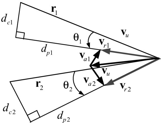
In the figure, the relative motion information with subscript i represents the information with respect to the ith aircraft. The relative velocity vectors of the UAS with respect to the first and second aircraft are obtained as
(7.21) ![]()
The distances to the close points of approach for each aircraft are given by
(7.22) ![]()
When the distances are smaller than the minimum separation within a specific time T at the same time:
(7.23) ![]()
there exist two conflicts, i.e. the UAS and aircraft are in multiple conflicts.
7.4 Conflict Resolution: Approach I
In this section, a conflict resolution algorithm for a single UAS with a constant speed is proposed. The resolution algorithm should guarantee a CAD of ![]() greater than or equal to the minimum separation of
greater than or equal to the minimum separation of ![]() . Whilst there might be many resolution velocity vectors meeting this requirement, we only consider the vector guaranteeing the following condition:
. Whilst there might be many resolution velocity vectors meeting this requirement, we only consider the vector guaranteeing the following condition:
(7.24) ![]()
As shown in Figure 7.7, if the relative velocity vector ![]() is aligned with the tangent to the minimum separation circle from the UAS, then the CAD will be equal to the minimum separation of
is aligned with the tangent to the minimum separation circle from the UAS, then the CAD will be equal to the minimum separation of ![]() .
.
Figure 7.7 Relative velocity for minimum separation (modified from [21])
If there exist uncertainties, an aircraft is manoeuvring, or both, this condition might be inappropriate for conflict resolution. Scaling up ![]() will resolve this problem because it results in a CAD bigger than the minimum separation. However, we leave this issue for future study.
will resolve this problem because it results in a CAD bigger than the minimum separation. However, we leave this issue for future study.
7.4.1 Collision Kinematics
For the conflict resolution, the direction of the relative velocity vector, ![]() , should become
, should become
(7.25) ![]()
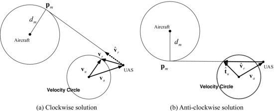
The resolution geometry for a clockwise solution is shown in Figure 7.8.
Figure 7.8 Conflict resolution geometry for clockwise rotation
The matching condition is thus derived as
where the sightline basis set ![]() is replaced by the separation basis set
is replaced by the separation basis set ![]() and
and
(7.27) ![]()
Calculating the ratio ![]() will determine the matching condition of the resolution geometry.
will determine the matching condition of the resolution geometry.
In order to derive the velocity ratio ![]() , the resolution geometry shown in Figure 7.9 is obtained by modifying the collision geometry.
, the resolution geometry shown in Figure 7.9 is obtained by modifying the collision geometry.
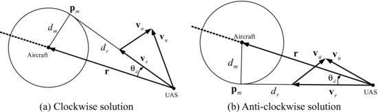
Figure 7.9 Geometry for minimum separation (modified from [21])
The figure shows that the original collision triangle has been modified to the resolution triangle given by ![]() , for both clockwise and anti-clockwise. This resolution triangle will maintain its orientation and shape in a similar manner to the impact triangle. The matching conditions for the clockwise and anti-clockwise solutions are shown in Figure 7.10.
, for both clockwise and anti-clockwise. This resolution triangle will maintain its orientation and shape in a similar manner to the impact triangle. The matching conditions for the clockwise and anti-clockwise solutions are shown in Figure 7.10.
Figure 7.10 Matching condition for minimum separation (modified from [21])
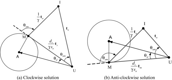
The vector sums for the UAS calculated with respect to the resolution triangle MIU yield the matching condition of the form
From equations (7.26) and (7.28), we have
(7.29) ![]()
Applying the cosine rule to the resolution geometry now gives
where
(7.31) ![]()
and ![]() denotes the angle between the sightline and the tangent line on the minimum separation circle from the UAS position. Note that
denotes the angle between the sightline and the tangent line on the minimum separation circle from the UAS position. Note that ![]() is either subtracted for a clockwise solution or added for an anti-clockwise solution. Now, we have
is either subtracted for a clockwise solution or added for an anti-clockwise solution. Now, we have
(7.32) ![]()
where
(7.33) 
Note that the geometry with respect to the sightline is now not fixed, but as the solution requires the relative velocity vector to lie along the tangent line from ![]() to
to ![]() , this line will not rotate. For the UAS and other aircraft with constant speed, this implies that the triangle
, this line will not rotate. For the UAS and other aircraft with constant speed, this implies that the triangle ![]() is fixed in shape and orientation, and will shrink as the UAS and aircraft approach each other. Hence the ratio
is fixed in shape and orientation, and will shrink as the UAS and aircraft approach each other. Hence the ratio ![]() will have a fixed solution, as will the angle subtended between the aircraft velocity vector and the tangent line
will have a fixed solution, as will the angle subtended between the aircraft velocity vector and the tangent line ![]() . Hence, a solution to equation (7.30) is calculated as
. Hence, a solution to equation (7.30) is calculated as
Given ![]() and
and ![]() in equation (7.34), the velocity ratio
in equation (7.34), the velocity ratio ![]() is obtained as
is obtained as
(7.35) ![]()
7.4.2 Resolution Guidance
Since the UAS heading angle is different from the desired one satisfying the matching condition in equation (7.28), it is essential to design an algorithm to regulate the heading angle at the desired angle. Let us define the desired UAS tangent vector as ![]() , then
, then
A geometric interpretation of equation (7.36) is reproduced in Figure 7.11.
Figure 7.11 Geometry interpretation of conflict resolution for clockwise rotation (modified from [20])
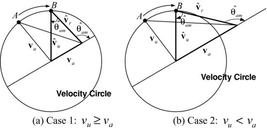
Figure 7.11 shows that as the geometry of the engagement changes due to mismatched UAS and aircraft tangent vectors, the solution ![]() will change and rotate around the circle. The figure also shows that the rotation of the solution vector
will change and rotate around the circle. The figure also shows that the rotation of the solution vector ![]() and the rotation of the sightline vector
and the rotation of the sightline vector ![]() are related. In moving from solution A to solution B, the solution angle
are related. In moving from solution A to solution B, the solution angle ![]() increases.
increases.
Minimum separation can be met by regulating the heading error, ![]() :
:
(7.37) ![]()
where ![]() and
and ![]() are the direction angles of the desired UAS tangent vector
are the direction angles of the desired UAS tangent vector ![]() and the UAS tangent vector
and the UAS tangent vector ![]() . The regulating algorithm of the heading angle can be determined by use of a simple Lyapunov function V of the form
. The regulating algorithm of the heading angle can be determined by use of a simple Lyapunov function V of the form
(7.38) ![]()
The time derivative of the Lyapunov candidate function V is given by
(7.39) ![]()
For stability, it is required that
(7.40) ![]()
From the definition of ![]() , we have
, we have
(7.41) ![]()
The first time derivative of the matching condition for minimum separation is obtained as
This means
From the definition of ![]() , we have
, we have
(7.44) ![]()
where
(7.45) ![]()
Here ![]() is the sightline angle. Since
is the sightline angle. Since ![]() for a non-manoeuvring aircraft, equation (7.51) becomes
for a non-manoeuvring aircraft, equation (7.51) becomes
Substituting equation (7.46) into equation (7.43) yields
From the resolution geometry, ![]() is obtained as
is obtained as
Equation (7.47) can be rewritten as
(7.49) ![]()
Hence, a resolution guidance algorithm is proposed as
(7.52) ![]()
to give
(7.53) ![]()
which is negative semi-definite. The curvature of UAS, ![]() can be obtained from equation (7.50) and
can be obtained from equation (7.50) and
7.4.3 Analysis and Extension
Now, let us analyse the proposed conflict resolution algorithm. In order to investigate the feasibility of conflict resolution, we should examine the velocity vectors. If the desired relative velocity is realisable from the combination of UAS and aircraft velocity vectors, the resolution algorithm is feasible. Otherwise, it is infeasible. From equation (7.34), it is possible to investigate the feasibility of the avoidance solutions for the UAS with a constant speed.
Lemma 7.1 For constant ground speed of the UAS, ![]() , if it is greater than or equal to that of the aircraft,
, if it is greater than or equal to that of the aircraft, ![]() , then the conflict resolution algorithm is feasible and the desired relative speed
, then the conflict resolution algorithm is feasible and the desired relative speed ![]() is given by
is given by
where
(7.56) ![]()
Proof. Multiplying both sides of equation (7.34) by ![]() yields
yields
(7.57) ![]()
From the assumption that ![]() is greater than or equal to
is greater than or equal to ![]() , we have
, we have
(7.58) 
for any values of the angle ![]() . Since
. Since ![]() should be a positive value, equation (7.55) is true for
should be a positive value, equation (7.55) is true for ![]() . Hence, the resolution algorithm is feasible.
. Hence, the resolution algorithm is feasible.
Lemma 7.2 For constant ground speed ![]() of the UAS less than the aircraft speed
of the UAS less than the aircraft speed ![]() :
:
- if
 is less than zero, there is no feasible solution, i.e. the desired relative velocity which cannot be aligned along with the two tangent vectors;
 - if
 is equal to zero, there is only one feasible solution, i.e. one desired relative velocity vector can be aligned with a corresponding tangent vector;
 - if
 is greater than zero, there exist two feasible solutions, i.e. two relative velocity vectors can be aligned along the two tangent vectors.
Figure 7.12 shows an example in which only one avoidance solution is feasible.
As illustrated in Figure 7.12, only the anti-clockwise solution is feasible. Note that the velocity circle in this figure represents a feasible UAS heading for a constant speed: its radius is the UAS speed and its centre is in a velocity vector of the aircraft from the UAS position.
Figure 7.12 An example of the existence of one feasible solution
The desired heading angle of the UAS can be calculated simply from equation (7.36). Since there could be two possible solutions, the clockwise and anti-clockwise, we need to determine the turning direction of the UAS. Figure 7.13 represents two resolution velocity vectors for that, ![]() .
.
Figure 7.13 Geometry of UAS velocity for conflict resolution (from [20])
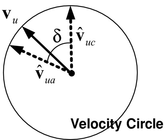
In the figure, ![]() and
and ![]() denote the desired UAS tangent vectors for the clockwise and anti-clockwise rotation, and
denote the desired UAS tangent vectors for the clockwise and anti-clockwise rotation, and ![]() represents the collision sector which lies between the two tangent vectors. Note that if the tangent vector is located inside the collision sector and TCPA is less than a specific time, then the UAS and aircraft are in conflict. On the other hand, the UAS and aircraft are not in conflict when the tangent vector is outside the sector. As shown in Figure 7.13, turning towards the vector
represents the collision sector which lies between the two tangent vectors. Note that if the tangent vector is located inside the collision sector and TCPA is less than a specific time, then the UAS and aircraft are in conflict. On the other hand, the UAS and aircraft are not in conflict when the tangent vector is outside the sector. As shown in Figure 7.13, turning towards the vector ![]() will make a clockwise turn and turning towards the vector
will make a clockwise turn and turning towards the vector ![]() will produce an anti-clockwise turn. If the UAS turns towards the closest vector, then it will produce a monotonically increasing CAD. To determine the turn direction, it is possible to consider several methods fulfilling the requirements – such as obeying the rules of the air, or allowing more efficient path following after the resolution manoeuvre. In this study, turning towards the closest vector is among the possible solutions considered.
will produce an anti-clockwise turn. If the UAS turns towards the closest vector, then it will produce a monotonically increasing CAD. To determine the turn direction, it is possible to consider several methods fulfilling the requirements – such as obeying the rules of the air, or allowing more efficient path following after the resolution manoeuvre. In this study, turning towards the closest vector is among the possible solutions considered.
Now, let us consider a simple scenario where the UAS and only two aircraft are in multiple conflicts. Figure 7.14(a, b) shows the velocity circles of the UAS with respect to the first and second aircraft, respectively.
Figure 7.14 Velocity circles against two aircraft
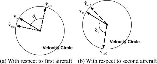
A conflict sector for multiple conflicts resolution ![]() is the union of two conflicts sectors
is the union of two conflicts sectors ![]() and
and ![]() :
:
(7.59) ![]()
In this scenario, the desired tangent vectors are ![]() and
and ![]() . Similarly, for n number of conflicts, the sector will be the union of all sectors:
. Similarly, for n number of conflicts, the sector will be the union of all sectors:
(7.60) ![]()
The heading angle of the relative vector for the resolution can be simply obtained as:
(7.61) ![]()
where n is the number of aircraft which are in conflict with the UAS, and the angles ![]() and
and ![]() are the angles
are the angles ![]() and
and ![]() with respect to the ith aircraft. The desired relative velocity for resolution of multiple conflicts is then chosen as the one satisfying the condition in equation (7.42). However, the decision to change direction needs to be carefully verified, because turning to the closest resolution vector from the current UAS velocity vector could result in a problem. Figure 7.15 illustrates.
with respect to the ith aircraft. The desired relative velocity for resolution of multiple conflicts is then chosen as the one satisfying the condition in equation (7.42). However, the decision to change direction needs to be carefully verified, because turning to the closest resolution vector from the current UAS velocity vector could result in a problem. Figure 7.15 illustrates.
Figure 7.15 A turning direction issue for multiple conflicts resolution (modified from [20])
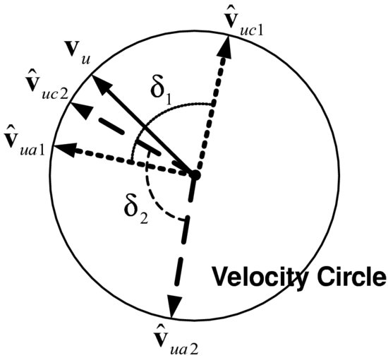
In the case shown in Figure 7.14, the UAS first tries to solve the second conflict and the velocity vector will be located outside ![]() , as shown in Figure 7.15. Since the proposed turning direction will rotate the velocity towards
, as shown in Figure 7.15. Since the proposed turning direction will rotate the velocity towards ![]() in this case, the UAS and aircraft will be in multiple conflicts again. Therefore, this problem might cause chattering on the resolution command and unsafe trajectories. In order to resolve this problem, simple decision-making is proposed. If a resolution manoeuvre does not satisfy the condition
in this case, the UAS and aircraft will be in multiple conflicts again. Therefore, this problem might cause chattering on the resolution command and unsafe trajectories. In order to resolve this problem, simple decision-making is proposed. If a resolution manoeuvre does not satisfy the condition
(7.62) ![]()
the UAS maintains the turning direction.
7.5 Conflict Resolution: Approach II
In the previous section, it was assumed that the ground speed of the UAS is constant to design a conflict resolution algorithm. Owing to this assumption, the resolution guidance controls the heading angle only. It also limits the feasibility region of the avoidance solutions: when the ground speed of the aircraft is greater than that of the UAS, some solutions are infeasible. An example scenario for an infeasible solution is shown in Figure 7.16.
Figure 7.16 Example geometry in which the clockwise solution is infeasible
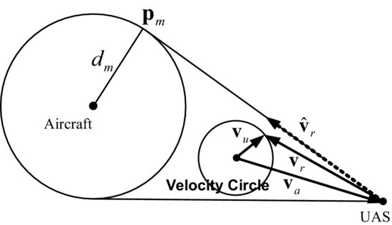
Note that the velocity circle can represent the feasibility of the solution: as illustrated in the figure, the desired relative velocity ![]() is unrealisable regardless of the UAS heading. We thus propose a resolution algorithm which can resolve this problem. Since the proposed resolution algorithm with constant speed can be used when the conflict solution is feasible, we only consider the case where the aircraft speed is greater than the UAS speed in this section.
is unrealisable regardless of the UAS heading. We thus propose a resolution algorithm which can resolve this problem. Since the proposed resolution algorithm with constant speed can be used when the conflict solution is feasible, we only consider the case where the aircraft speed is greater than the UAS speed in this section.
7.5.1 Resolution Kinematics and Analysis
As stated in Section 7.4, a relative velocity vector should be aligned with one of the two tangent vectors for conflict resolution. Controlling the speed with UAS heading could enlarge the feasibility region so as to generate a feasible solution as shown in Figure 7.17.
Figure 7.17 Concept of controlling heading and speed of UAS
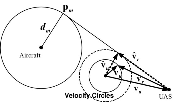
In the figure, the velocity circle with the solid line is the circle with the current UAS velocity and the dashed circle is a circle with a modified velocity vector. As depicted, the UAS is able to realise a desired relative velocity, ![]() , not with the current speed, but with an increased speed.
, not with the current speed, but with an increased speed.
There might be numerous avoidance solutions when the UAS speed can be controlled. Figure 7.18(a) shows a few possible solutions in a simple scenario.
Figure 7.18 Velocity relation for avoidance solutions
In order to determine the avoidance solution, let us investigate the velocity relation. The velocity relation with an arbitrary relative speed ![]() is given by
is given by
Since equation (7.63) can be rewritten as
(7.64) ![]()
we have
(7.65) ![]()
For aircraft with a constant speed, determining ![]() defines the desired UAS speed and consequently the avoidance solution. The minimum UAS speed for the conflict resolution can be derived from the following condition:
defines the desired UAS speed and consequently the avoidance solution. The minimum UAS speed for the conflict resolution can be derived from the following condition:
If ![]() , the minimum UAS speed satisfying equation (7.66) is the aircraft speed. Otherwise, the minimum speed is obtained as
, the minimum UAS speed satisfying equation (7.66) is the aircraft speed. Otherwise, the minimum speed is obtained as
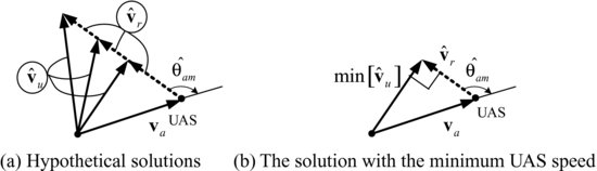
A geometric interpretation of equation (7.67) is shown in Figure 7.18(b): the relative speed yielding the minimum UAS speed is given by
(7.68) ![]()
As stated, the resolution algorithm controlling the speed and heading will be implemented only when the avoidance solution is infeasible. In this case, the UAS speed must be increased to make the solution feasible, as shown in Figure 7.17. In this study, therefore, the avoidance solution is derived from the minimum UAS ground speed to minimise deviation from the current speed of UAS resulting in the minimum fuel consumption. Note that the UAS velocity is likely to be chosen for a certain mission, thus the resolution algorithm obtained from the minimum UAS speed would also be desirable for mission accomplishment.
If the minimum solution among the desired UAS speeds is greater than the maximum bound of the UAS speed, there is no feasible solution for conflict resolution. In this case, the best resolution manoeuvre is to maximise the speed and align the UAS heading with the desired velocity vector as closely as possible.
7.5.2 Resolution Guidance
Owing to the speed and heading of UAS which are different from the desired ones for conflict resolution, it is necessary to develop a regulation algorithm – termed ‘resolution guidance’ in this study. In order to design an algorithm, the Lyapunov stability theory is used again. The stability of the conflict resolution algorithm can be determined by implementing a simple Lyapunov candidate function V, of the form
(7.69) ![]()
where
(7.70) ![]()
The time derivative of the function V is given by
(7.71) ![]()
In order to guarantee the stability, the resolution guidance must satisfy the following equation:
(7.72) ![]()
From equation (7.67), the time derivative of ![]() is derived as
is derived as
Substituting equations (7.46) and (7.48) into equation (7.73) yields
(7.74) ![]()
Hence, we have
(7.75) ![]()
For the desired UAS speed equal to that of the aircraft, we have
(7.76) ![]()
As shown in Figure 7.18(b), ![]() is a right angle and its first time derivative is zero. Therefore, the resolution guidance algorithm is proposed as
is a right angle and its first time derivative is zero. Therefore, the resolution guidance algorithm is proposed as
(7.77) 
to give
(7.78) ![]()
for ![]() and
and ![]() . The curvature of the UAS,
. The curvature of the UAS, ![]() , can be obtained from equation (7.54) and the tangential acceleration is given from
, can be obtained from equation (7.54) and the tangential acceleration is given from
(7.79) ![]()
7.6 CD&R Simulation
In this section, the performance and reliability of the proposed CD&R algorithms are investigated using numerical examples. For the nonlinear simulation, it is assumed that UAS are able to obtain the following motion information of aircraft by any means:
- position vector;
- velocity vector.
Furthermore, the look-ahead time T is selected as 3 minutes and 3 km is considered as a minimum separation distance. Note that the FAA classified minimum vertical and horizontal separation distances considering several standards: minimum horizontal separation for aircraft safety is 5 nautical mile (nm) in the en-route environment and 3 nm in the terminal environment; minimum vertical separation is currently 1,000 ft at flight levels below 41,000 ft. The UAS heads to a waypoint of (20 km, 20 km) and its initial position and heading angle of UAS are (0 km, 0 km) and 0 degree.
7.6.1 Simulation Results: Approach I
For the numerical examples to examine the performance of the first approach, two scenarios are considered. In the scenarios, it is assumed that the initial ground speed of the UAS is 100 m/s and the physical constraints imposed on the UAS are given in Table 7.1.
Table 7.1 Physical constraints of UAS for the first resolution approach
The initial conditions of intruders (aircraft) are represented in Table 7.2.
Table 7.2 Initial conditions of aircraft for the first resolution approach

Aircraft are non-manoeuvring in the first scenario, whereas in the second scenario they are manoeuvring with a constant turn rate give as
(7.80) ![]()
Whilst the first scenario is to verify the performance of the conflict detection and the first resolution algorithms, the second scenario is to check their performance when the non-manoeuvring assumption is no longer valid. Note that the conflict detection and first resolution algorithms are derived with a constant UAS speed. The original trajectories without conflict resolution are shown in Figure 7.19.
Figure 7.19 Original trajectories: the first resolution approach
In this figure, the solid line represents the trajectory of the UAS, solid lines and circles with markers show the trajectories of aircraft and the minimum separation circles at the minimum distances from the UAS, and a diamond shape at (20 km, 0 km) illustrates the waypoint the UAS heads to. Note that the UAS shapes are depicted at the closest points from the aircraft, thus the UAS is in conflict with the aircraft if any UAS is located in the minimum separation circles. In the two scenarios, UAS is in conflicts with the first, second and fourth aircraft. As shown in Figure 7.19, one UAS and four aircraft are initially distributed over a rectangular air space of 20 km by 10 km. Since the simulated space is more stressed than that in a hypothetical conflict situation, it will allow the rigorous performance evaluation of the proposed CD&R algorithms.
In order to resolve the multiple conflicts, the conflict detection algorithm and the first resolution approach are implemented into UAS. The minimum distances between the UAS and aircraft are always greater than the minimum safe separation of 3 km as represented in Table 7.3, so the proposed algorithms effectively detect and resolve the conflicts.
Table 7.3 Minimum relative distances of aircraft from the UAS: the first resolution approach
| Intruder | First scenario | Second scenario |
| Aircraft 1 | 4.2040 km | 4.0679 km |
| Aircraft 2 | 3.2297 km | 3.1219 km |
| Aircraft 3 | 3.0752 km | 3.0220 km |
| Aircraft 4 | 3.0680 km | 3.0693 km |
Simulation results in the first scenario are shown in Figure 7.20.
Figure 7.20 Results in the first scenario for the first resolution appoach
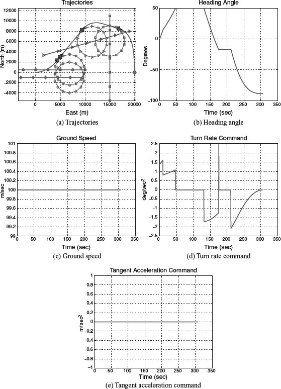
Figure 7.21 Results in the second scenario for the first resolution approach
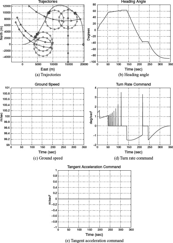
As shown in Figure 7.20(a, b, d), not only can the first resolution approach avoid the collision, but also the heading change of the UAS is smooth. It is also shown in Figure 7.20(c, e) that the ground speed of the UAS is constant. Figure 7.21 illustrates the simulation results in the second scenario.
As depicted in these figures, the proposed algorithm resolves conflicts and maintains a constant ground speed. However, the turn rate command is spiky because the detection algorithm is derived against non-manoeuvring: aircraft manoeuvre will generate conflict conditions resulting from the altered aircraft heading.
7.6.2 Simulation Results: Approach II
In the numerical examples for the performance evaluation of the second approach, we assume that the initial ground speed of the UAS is 50 m/s and the physical constraints of the UAS are given in Table 7.4.
Table 7.4 Physical constraints of UAS for the first resolution approach
Table 7.5 represents the initial conditions of the aircraft.
Table 7.5 Initial conditions of aircraft for the first resolution approach
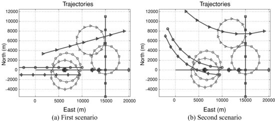
Note that, unlike the numerical examples for the first resolution approach, the UAS speed is less than that of the aircraft. The turn rates of the aircraft for each scenario are the same as those for the first resolution approach. In these scenarios, without the resolution algorithm, conflicts exist between the UAS and the first, second and fourth aircraft as shown in Figure 7.22.
Figure 7.22 Original trajectories: the second resolution approach
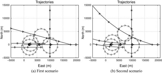
Table 7.6 represents the minimum distances between the UAS and the aircraft. From the distances which are bigger than the safe distance, it is shown that the conflicts detection and the second resolution approach work effectively.
Figure 7.23 shows the simulation results in the first scenario.
Since there was no feasible avoidance solution at the beginning of the simulation, the resolution algorithm increases the UAS speed. The second scenario is considered to check the effect when the assumption of non-manoeuvring aircraft is invalid and its results are illustrated in Figure 7.24.
Table 7.6 Minimum relative distances of aircraft from the UAS: the second resolution approach
| Intruder | First scenario | Second scenario |
| Aircraft 1 | 3.5952 km | 3.5689 km |
| Aircraft 2 | 3.0096 km | 3.0980 km |
| Aircraft 3 | 5.2482 km | 4.1128 km |
| Aircraft 4 | 3.0177 km | 3.0607 km |
Figure 7.23 Results in the first scenario for the second resolution approach
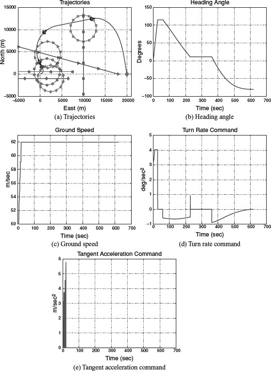
Figure 7.24 Results in the second scenario for the second resolution approach
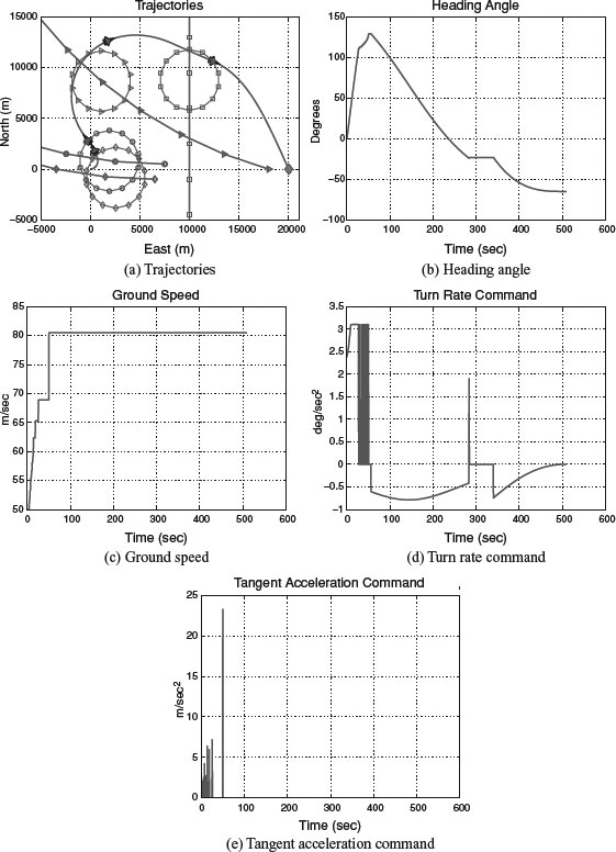
The simulation results show that the second resolution approach successively resolves the conflicts. In the second scenario, the UAS speed is again increased to make an unrealisable solution feasible. Moreover, similar to the first resolution approach in the second scenario, the aircraft manoeuvre results in chattering on the turn rate command. In Figure 7.23(e) and Figure 7.24(e), the tangent acceleration commands seem to be chattering. Therefore, we check the command profiles in a smaller time window and they are depicted in Figure 7.25.
Figure 7.25 Tangent acceleration command in a time window
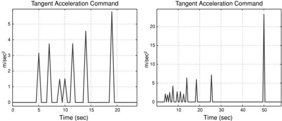
As shown in Figure 7.25, the tangent acceleration command is not in fact chattering.
7.7 Conclusions
In this chapter, a UAS conflict detection algorithm and two resolution algorithms have been introduced based on the differential geometry concepts. To develop all algorithms, it is assumed that aircraft are non-manoeuvring. The closest approach distance (CAD) and time to closest point of approach (TCPA) allow the detection algorithm to define the conflict. Whilst the first resolution algorithm controls the UAS heading only, the second algorithm controls both the ground speed and the heading. The feasibility and performance of two algorithms were also mathematically analysed. If the aircraft speed is greater than the UAS speed, the constant speed of the UAS may lead to infeasible solutions. The second algorithm resolves this problem and consequently expands the feasibility region by controlling the UAS speed. We also extended the proposed algorithms for the multiple conflicts in which a UAS and many aircraft are in danger of collision at the same time. The performance of the detection and resolution algorithms was also illustrated and validated through numerical simulations. The results of the nonlinear simulation have shown that the proposed algorithm performs effectively not only for non-manoeuvring aircraft, but also for manoeuvring aircraft. The analysis did not include the UAS dynamics and this, together with the extension to 3D, will be the subject of future study.
References
1. Han, S. C. and Bang, H. C., ‘Proportional navigation-based optimal collision avoidance for UASs’, Proceedings of the 2nd International Conference on Autonomous Robots and Agents, Palmerston North, New Zealand, 2004.
2. Tomlin, C., Pappas, G. J., and Sastry, S., ‘Conflict resolution for air traffic management: a study in multi-agent hybrid systems’, IEEE Transactions on Automatic Control, 43(4), 509–521, 1998.
3. RTCA TF 3, Final report of RTCA Task Force 3: Free flight implementation, RTCA Task Force 3, RTCA Inc., Washington, DC, 1995.
4. Kuchar, J. and Yang, L., ‘Review of conflict detection and resolution modeling methods’, IEEE Transactions on Intelligent Transportation Systems, 1(4), 179–189, 2000.
5. Khatib, O. and Burdick, A., ‘Unified approach for motion and force of robot manipulators’, IEEE Journal of Robotics and Automation, 3(1), 43–53, 1987.
6. Passino, K. M., ‘Bridging the gap between conventional and intelligent control’, Control Systems Magazine, IEEE, 13(3), 12–18, 1993.
7. Tang, P., Yang, Y., and Li, X., ‘Dynamic obstacle avoidance based on fuzzy inference and transposition principle for soccer robots’, Proceedings of 10th International Conference on Fuzzy Systems, Melbourne, Victoria, Australia, 2001.
8. Rathbun, D., Kragelund, S., Pongpunwattana, A., and Capozzi, B., ‘An evolution based path planning algorithm for autonomous motion of a UAS through uncertain environments’, Proceedings of IEEE Digital Avionics Systems Conference, 2002.
9. Ghosh, R. and Tomlin, C., ‘Maneuver design for multiple aircraft conflict resolution’, Proceedings of American Control Conference, Chicago, IL, 2000.
10. Kumar, B. A. and Ghose, D., ‘Radar-assisted collision avoidance/guidance strategy for planar flight’, IEEE Transactions on Aerospace and Electronic System, 37(1), 77–90, 2001.
11. Sunder, S. and Shiller, Z., ‘Optimal obstacle avoidance based on the Hamilton–Jacobi–Bellman equation’, IEEE Transactions on Robotics and Automation, 13(2), 305–310, 1997.
12. Kuchar, J., Andrews, J., Drumm, A., Hall, T., Heinz, V., Thompson, S., and Welch, J., ‘A safety analysis process for the traffic alert and collision avoidance system (TCAS) and see-and-avoid systems on remotely piloted vehicles’, Proceedings of AIAA 3rd ‘Unmanned Unlimited’ Technical Conference, Workshop and Exhibit, Chicago, IL, 2004.
13. Cho, S. J., Jang, D. S., and Tahk, M. J., ‘Application of TCAS-II for unmanned aerial vehicles’, Proceedings of 2005 JSASS-KSASS Joint Symposium on Aerospace Engineering, Nagoya, Japan, 2005.
14. Asmat, J., Rhodes, B., Umansky, J., Villavicencio, C., Yunas, A., Donohue, G., and Lacher, A., ‘UAS safety: unmanned aerial collision avoidance system (UCAS)’, Proceedings of the 2006 Systems and Information Engineering Design Symposium, Charlottesville, VA, 2006.
15. DeGarmo, M. T., Issues Concerning Integration of Unmanned Aerial Vehicles in Civil Airspace, MP 04W0000323, MITRE, November, 2004.
16. Hedlin, S., Demonstration of Eagle MALE UAS for Scientific Research, Swedish Space Corporation Mattias Abrahamsson, Swedish Space Corporation, 2002. Available online at: http://www.neat.se/information /papers/NEAT_paper_Bristol_2003.pdf.
17. Kayton, M. and Fried, W. R., Avionics Navigation Systems, John Wiley & Sons, New York, 1996.
18. Dowek, G. and Muñoz, C., ‘Conflict detection and resolution for 1, 2, … , N aircraft’, Proceedings of the 7th AIAA Aviation Technology, Integration and Operations Conference, Belfast, Northern Ireland, 2007.
19. Galdino, A., Muñoz, C., and Ayala, M., ‘Formal verification of an optimal air traffic conflict resolution and recovery algorithm’, Proceedings of the 14th Workshop on Logic, Language, Information and Computation, 2007.
20. Shin, H. S., White, B. A., and Tsourdos, A., ‘Conflict detection and resolution for static and dynamic obstacles’, Proceedings of AIAA GNC 2008, August 2008, Honolulu, HI, AIAA 2008-6521 .
21. White, B. A., Shin, H. S., and Tsourdos, A., ‘UAV obstacle avoidance using differential geometry concepts’, IFAC World Congress 2011, Milan, Italy, 2011.