Chapter 1

Introducing Signals and Systems

In This Chapter

Figuring out the math you need for signals and systems work

Determining the different types of signals and systems

Understanding signal classifications and domains

Checking out possible products with behavioral level modeling

Looking at real products as signals and systems

Using open-source computer tools to check your work

Which came first: the signal or the system? Before you answer, you may want to know that by system, I mean a structure or design that operates on signals. You live and breathe in a sea of signals, and systems harness signals and put them to work. So which came first, you think? It may not really matter, but I’m guessing — as I smooth out a long imaginary philosopher-type beard — that signals came first and then began passing through systems.

But I digress. The study of signals and systems as portrayed in this book centers on the mathematical modeling of both signals and systems. Mathematical modeling allows an engineer to explore a variety of product design approaches without committing to costly prototype hardware and software development. After you tune your model to produce satisfactory results, you can implement your design as a prototype. And at some point, real signals (and sometimes math-based simulations) test the system design before full implementation.

When studying signals and systems, it’s easy to get mired in mathematical details and lose sight of the big picture — the functional systems of your end result. So try to remember that, at its best, signals and systems is all about designing and working with products through applied math. Math is the means, not the star of the show.

Two broad classes of signals are those that are continuous functions of time t and those that are discrete functions of time index n. Throughout this book, I separate information on continuous- and discrete-time signals and systems. In this chapter, I introduce simple continuous and discrete signals and the corresponding systems. I also point out some of the distinguishing characteristics of signal types.

Before getting started, I want to mention that signals as functions of time are how most people experience the real world of computer and electronic engineering, yet transforming signals and systems to other domains — specifically, the frequency, s-, and z-domains — and back again is quite beneficial in some situations. I touch on the transformation of signals and systems in this chapter and dig into the details in Parts III and IV.

In this chapter, I also cover the important role of computer tools in signals and systems problem solving and tell you how to use a few specific open-source programs. If you want to set up these freely available tools on your computer, you can follow along when I describe specific functions that enable you to check your work or work more efficiently — after you get a handle on core concepts and techniques.

Applying Mathematics

Anyone aspiring to a working knowledge of signals and systems needs a solid background in math, including these specific concepts:

Calculus of one variable

Integration and differentiation

Differential equations

To actually implement designs that center on signals and systems, you also need a background in these subjects:

Electrical/electronic circuits

Computer programming fundamentals, such as C/C++ and Java

Analysis, design, and development software tools

Programmable devices

Many signals and systems designers rely on modeling tools that use a matrix/vector language or class library for numerics and a graphics visualization capability to allow for rapid prototyping. I use numerical Python for examples in this book; other languages with similar syntax include MATLAB and NI LabVIEW MathScript.

---

---

With so many electrical engineering solutions being software-based today — versus a matter of analog circuitry (see nearby sidebar “Finding perspective on analog processing”) — a system designer can also be the implementer. This leap requires only simulation code to be transformed into the implementation language, such as Verilog or C/C++.

Working pencil-and-paper solutions for signals and systems coursework requires a good scientific calculator. I recommend a calculator that supports complex arithmetic operations, using the minimum number of keystrokes. At minimum, your calculator needs to have trig, log, and exponential functions for signals and systems work.

Getting Mixed Signals . . . and Systems

Signals come in two flavors: continuous and discrete. It’s the same story with systems. In other words, some signals — and some systems — are active all the time; others aren’t. In this section, I describe continuous and discrete signals along with the corresponding systems. I also tell you how to classify certain signals and systems based on their most basic properties.

Going on and on and on

Continuous-time signals and systems never take a break. When a circuit is wired up, a signal is there for the taking, and the system begins working — and doesn’t stop. Keep in mind that I use the term signal here loosely; any one specific signal may come and go, but a signal is always present at each and every time instant imaginable in a continuous-time system.

Continuous-time signals

Continuous signals function according to time t. A sinusoidal function of time is one of the most basic signals. The mathematical model for a sinusoid signal is , where A is the signal amplitude, is the signal frequency, and is the signal phase shift. The independent variable is time t. If you’re curious about the first peak of x (t) occuring at 3/16, notice that this occurs when the argument of the cosine is 0 — the is, or .

I cover this signal in detail in Chapter 3, but to help you get acquainted, check out the plot of a sinusoid signal in Figure 1-1.

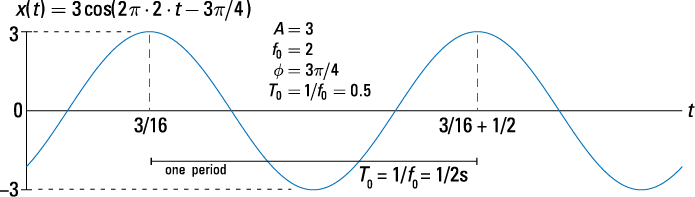
Figure 1-1: The plot of a sinusoidal signal.

The amplitude of this signal is 3, the frequency is 2 Hz, and the phase shift is rad.

Continuous-time systems

Systems operate on signals. In mathematical terms, a system is a function or operator, , that maps the input signal to output signal .

An example of a continuous-time system is the electronic circuits in an amplifier, which has gain 5 and level shift 2: .

See a block diagram representation of this simple system in Figure 1-2.

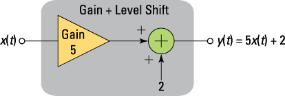
Figure 1-2: A simple continuous-time system model.

Building an amplifier that corresponds to this mathematical model is another matter entirely. You can create a simple electronic circuit, but it will have limitations that the math model doesn’t have. It’s up to you, as an electronic engineer, to refine the model to accurately reflect the level of detail needed to assess overall performance of a design candidate.

Working in spurts: Discrete-time signals and systems

Discrete-time signals and systems march along to the tick of a clock. Mathematical modeling of discrete-time signals and systems shows that activity occurs with whole number (integer) spacing, but signals in the real world operate according to periods of time, or the update rate also known as the sampling rate. Discrete-time signals, which can also be viewed as sequences, only exist at the ticks, and the systems that process these signals are, mathematically speaking, resting in the periods between signal activity.

Systems take inputs and produce outputs with the same clock tick, generally speaking. Depending on the nature of the digital hardware and the complexity of the system, calculations performed by the system continue — between clock ticks — to ensure that the next system output is available at the next tick when a new signal sample arrives at the input.

Discrete-time signals

Discrete-time signals are a function of time index n. Discrete-time signal , unlike continuous-time signal , takes on values only at integer number values of the independent variable n. This means that the signal is active only at specific periods of time. Discrete-time signals can be stored in computer memory because the number of signal values that need to be stored to represent a finite time interval is finite.

The following simple signal, a pulse sequence, is shown in Figure 1-3 as a stem plot — a plot where you place vertical lines, starting at 0 to the sample value, along with a marker such as a filled circle. The stem plot is also known as a lollipop plot — seriously.

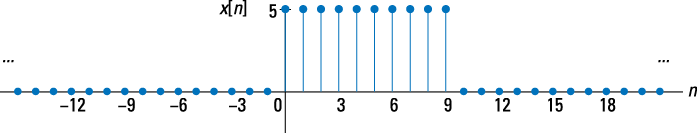
Figure 1-3: A simple discrete-time signal.

The stem plot shows only the discrete values of the sequence. Find out more about discrete-time signals in Chapter 4.

Discrete-time systems

A discrete-time system, like its continuous-time counterpart, is a function, , that maps the input to the output . An example of a discrete-time system is the two-tap filter:

The term tap denotes that output at time instant n is formed from two time instants of the input, n and n – 1. Check out a block diagram of a two-tap filter system in Figure 1-4.

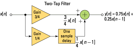
Figure 1-4: A simple discrete-time system model.

In words, this system scales the present input by 3/4 and adds it to the past value of the input scaled by 1/4. The notion of the past input comes about because is lagging one sample value behind . The term filter describes the output as an averaging of the present input and the previous input. Averaging is a form of filtering.

Classifying Signals

Signals, both continuous and discrete, have attributes that allow them to be classified into different types. Three broad categories of signal classification are periodic, aperiodic, and random. In this section, I briefly describe these classifications (find details in Chapters 3 and 4).

Periodic

Signals that repeat over and over are said to be periodic. In mathematical terms, a signal is periodic if

The smallest T or N for which the equality holds is the signal period. The sinusoidal signal of Figure 1-1 is periodic because of the property of cosine. The signal of Figure 1-1 has period 0.5 seconds (s), which turns out to be the reciprocal of the frequency Hz. The square wave signal of Figure 1-5a is another example of a periodic signal.

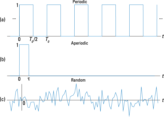
Figure 1-5: Examples of signal classifications: periodic (square wave) (a), aperiodic (rectangular pulse) (b), and random (noise) (c).

Aperiodic

Signals that are deterministic (completely determined functions of time) but not periodic are known as aperiodic. Point of view matters. If a signal occurs infrequently, you may view it as aperiodic. The rectangular pulse of duration shown in Figure 1-5b is an aperiodic signal.

Random

A signal is random if one or more signal attributes takes on unpredictable values in a probability sense (you love statistics, right?).

The full mathematical description of random signals is outside the scope of this book, but here are two good examples of a random signal:

The noise you hear when you’re between stations on an FM radio. See a waveform representation of this noise in Figure 1-5c.

Speech: If you try to capture audio samples on a computer of someone speaking the word hello over and over, you’ll find that each capture looks a little different.

Engineers working with communication receivers are concerned with random signals, especially noise.

Signals and Systems in Other Domains

Most of the signals you encounter on a daily basis — in computers, in wireless devices, or through a face-to-face conversation — reside in the time domain. They’re functions of independent variable t or n. But sometimes when you’re working with continuous-time signals, you may need to transform away from the time domain (t) to either the frequency domain () or the s-domain (s). Similarly, for discrete-time signals, you may need to transform from the discrete-time domain (n) to the frequency domain () or the z-domain (z).

Systems, continuous and discrete, can also be transformed to the frequency and s- and z-domains, respectively. Signals can, in fact, be passed through systems in these alternative domains. When a signal is passed through a system in the frequency domain, for example, the frequency domain output signal can later be returned to the time domain and appear just as if the time-domain version of the system operated on the signal in the time domain.

This section briefly explores the world of signals and systems in the frequency, s-, and z-domains. Find more on these alternative domains in Chapters 13 and 14.

Viewing signals in the frequency domain

The time domain is where signals naturally live and where human interaction with signals occurs, but the full information for a signal isn’t always visible in that space. Consider the sum of a two-sinusoids signal (as depicted in Figure 1-6):

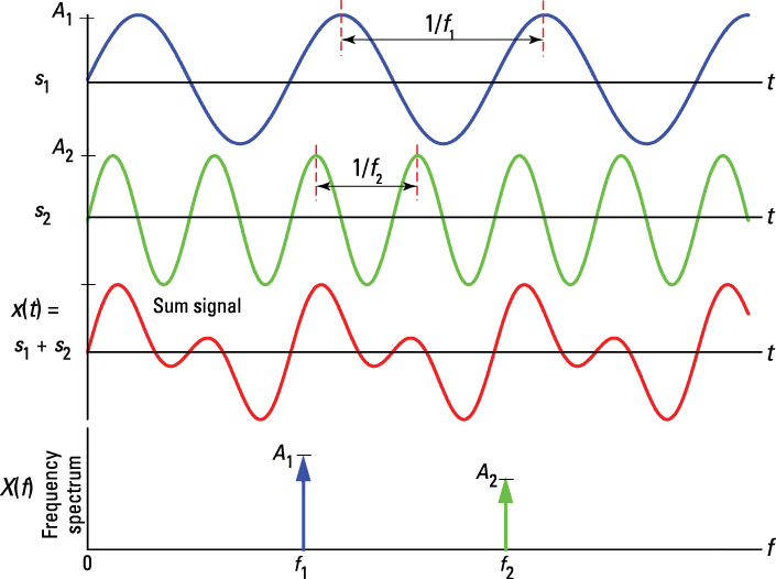
Figure 1-6: The frequency domain view for a sum of a two-sinusoids signal.

The top waveform plot, denoted s1, is a single sinusoid at frequency f1 and peak amplitude A1. The waveform repeats every period T1 = 1/f1. The second waveform plot, denoted s2, is a single sinusoid at frequency f2 > f1 and peak amplitude A2 < A1. The sum signal, s1 + s2, in the time domain is a squiggly line (third waveform plot), but the amplitudes and frequencies (periods) of the sinusoids aren’t clear here as they are in the first two plots. The frequency spectrum (bottom plot) reveals that is composed of just two sinusoids, with both the frequencies and amplitudes discernible.

Think about tuning in a radio station. Stations are located at different center frequencies. The stations don’t interfere with one another because they’re separated from each other in the frequency domain. In the frequency spectrum plot at the bottom of Figure 1-6, imagine that f1 and f2 are the signals from two radio stations, viewed in the frequency domain. You can design a receiving system to filter s1 from s1 + s2. The filter is designed to pass s1 and block s2. (I cover filters in Chapter 9.)

Use the Fourier transform to move away from the time domain and into the frequency domain. To get back to the time domain, use the inverse Fourier transform. (Find out more about these transforms in Chapter 9.)

Traveling to the s- or z-domain and back

From the time domain to the frequency domain, only one independent variable, , exists. When a signal is transformed to the s-domain, it becomes a function of a complex variable . The two variables (real and imaginary parts) describe a location in the s-plane.

In addition to visualization properties, the s-domain reduces differential equation solving to algebraic manipulation. For discrete-time signals, the z-transform accomplishes the same thing, except differential equations are replaced by difference equations. Did you think going to the z-domain meant taking a nap? Details on difference equations begin in Chapter 7.

Testing Product Concepts with Behavioral Level Modeling

Computer and electrical engineers provide society with a vast array of products — ranging from cellphones and high-definition televisions to powerful computers with high resolution displays that are small and lightweight. The mystery of how brilliant people come up with world-changing ideas may never be solved, but after an idea is out there, engineers work through a process that allows them to test, or model, potential solutions to find out whether the idea is likely to work in the real world. For products that rely on signal processing, engineers use signals and system modeling and analysis to reveal what’s possible.

When you’re trying to quickly prove a solution approach, you’ll often turn to behavioral level modeling of certain elements of the overall system to avoid low-level implementation details. For example, a subsystem design may require knowledge of a signal parameter (such as amplitude or frequency) to function. At first, you may assume that the parameter is well known. Later, you add low-level details to estimate (not perfectly) the parameter. As your confidence and understanding grows, you represent the low-level details in the model and actual implementation becomes possible.

Behavioral level modeling also applies when you need to model physical environments that lie outside a design but are needed to evaluate performance under realistic scenarios.

In this section, I describe the role of abstraction as a means to generate preliminary concepts and then work those concepts into a top-level design. The top-level design becomes a detailed plan as you work down to implementation specifics. Mathematical modeling is a thread running through the entire process, so you come to rely on it.

Staying abstract to generate ideas

Behavioral level modeling isn’t void of hardware constraints and realities, but it requires a certain level of abstraction to allow preliminary concept solutions to materialize quickly. Behavioral level models depend on applied mathematics.

In other words, computer and electronic engineers don’t frequently handle actual hardware and devices used for an implementation. The model of the hardware is what’s important at this point. The engineer’s job is to conceptualize systems and subsystems through a framework of mathematical concepts, and abstraction provides great creative freedom to explore the possibilities.

Suppose you seek a new design for an existing system to improve performance. You hope to make such improvements with new device technology. You don’t want to get bogged down in all the details of how to interface this device into the current design, so you move up in abstraction with a model to quickly find out how much you can improve performance with a new design. If adequate improvement potential doesn’t exist, then you settle down and investigate other options. Rinse, lather, and repeat.

Keep in mind that improved performance isn’t always the primary objective of signals and systems modeling. Sometimes, a design is driven by cost, availability of materials, manufacturing processes, and time to market, or some other consideration.

Working from the top down

A design that relies on signals and systems starts from a top-level view and works down to the nitty-gritty details of final implementation. Analysis and simulation performed at the top level depends on behavioral level modeling. The model is ultimately broken into subsystems for testing and refinement, and then the system comes together again before implementation.

Typically, your task as an electronic engineer is to create some new or enhanced functionality for a computer- or electrical-based product. For example, you may need to support a new radio interface due to recent standard updates. At first, the changes may seem simple and straightforward, but as you dig into the work, you may begin to see that the changes require significant adjustments in signal processing algorithms. This means that the new radio interface will require a few totally new designs, so you need to model and simulate various implementation approaches to find out what’s likely to work best.

Relying on mathematics

Many people write off signals and systems as a pile of confusing math, and they run for the hills. True, the math can be intimidating at first, but the rewards of seeing your finely crafted mathematical model lead the way to a shipping product is worth the extra effort — at least I think so. In the end, the math is on your side. It’s the only way to model concepts that function properly in the real world.

My go-to approach when a problem seems unsolvable: Take it slow and steady. If a solution isn’t clear after you think about the problem for a while, walk away and come back to it later. Practice and experience with various problem-solving techniques and options help, so try to work as many types of problems as you can — especially in the areas you feel the most discomfort. Eventually, a solution reveals itself.

When possible, verify your solutions by using computer analysis and simulation tools. In this book, I use Python with the numerical support and visualization capabilities of PyLab (NumPy, SciPy, matplotlib) and the IPython environment to perform number-crunching analysis and simulations. For problems involving more symbolic mathematics, I use the computer algebra system (CAS) provided by Maxima.

Exploring Familiar Signals and Systems

I’m guessing you have some level of familiarity with consumer electronics, such as MP3 music players, smartphones, and tablet devices, and realize that these products rely on signals and systems. But you may take for granted the cruise control in your car. In this section, I point out the signals and systems framework in familiar devices at the block diagram level — a system diagram that identifies the significant components inside rectangular boxes, interconnected with arrows that show the direction of signal flow. The block diagram expresses the overall concept of a system without intimate implementation details.

MP3 music player

Signals and systems are operating in all the major peripherals of the music player — even in the processor. In reality, signals are in every part of the system, but I exclude pure digital signals in this example, so I don’t address memory. The processor runs an operating system (OS); under that OS, tasks perform digital signal processing (DSP) algorithms for streaming audio and image data. Note that this book is focused on one-dimensional signals only.

Find a top-level block diagram of an MP3 device in Figure 1-7. All the peripheral blocks (the blocks that sit outside the processor block) contain a combination of continuous- and discrete-time systems. You stream digital music in real time from memory in a compressed format. The processor has to decompress the audio stream into signal sample values (a discrete-time signal) to send to the audio codec. The audio codec contains a digital-to-analog converter (DAC) that converts the discrete-time signal to a continuous-time signal.

The Wi-Fi and Bluetooth radios (blocks with antennas) interface to the processor with digital data but interface to the antenna by using a continuous-time signal at a frequency of 2.4 GHz. The sensors’ block acquires analog signals from the environment, temperature, light level, and acceleration in three dimensions.

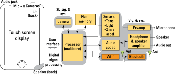
Figure 1-7: MP3 music player block diagram.

Smartphone

The structure of a smartphone is similar to an MP3 music player, but a smartphone also has a global positioning receiver (GPS) and multiband radio blocks that send and receive continuous-time signals from base stations (antenna sites) of a cellular network. The GPS receiver acquires signals from multiple satellites to get your latitude and longitude. The primary purpose of the GPS in most smartphones is to provide location information when placing an emergency call (E911).

Check out a block diagram of a smartphone in Figure 1-8. Four antennas are shown, but only a single multiband antenna is employed in most models, so only a single antenna structure is really needed.

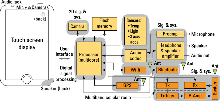
Figure 1-8: Smartphone block diagram.

The multiband cellular radio subsystem is thick with signals and systems. The multiband digital communications transmitter (tx) and receiver (rx) allows the smartphone to be backward compatible with older technologies as well as with the newest high-speed wireless data technologies. This transmitter and receiver enable the product to operate throughout the world. A smartphone is overflowing with signals and systems examples!

Automobile cruise control

I think all new automobiles come equipped with a cruise control system now. This is good news because this feature may keep you from getting a speeding ticket when you’re driving long distances on the interstate. It’s also great for getting better gas mileage. But I’m no sales guy for cruise control. I just think this product is interesting from a signals and systems standpoint.

Figure 1-9 shows a block diagram of a cruise control system. Cruise control involves both electrical and mechanical signals and systems. The controller is electrical and the plant, the system being controlled, is the car. Wind and hills are disturbance signals, which thwart the normal operation of the control system. The controller puts out a compensating signal to the throttle to overcome wind resistance (an opposing force) and the force of gravity when going up and down hills. The error signal that follows the summing block is driven to a very small value by the action of the feedback loop. This means that the output velocity tracks the reference velocity. This is exactly what you want. For a more detailed look at cruise control, check out the case studies at www.dummies.com/extras/signalsandsystems.

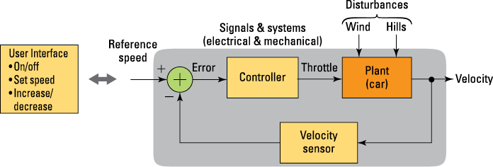
Figure 1-9: Block diagram of an automobile cruise control system.

Using Computer Tools for Modeling and Simulation

Today’s technology-based solutions are rarely built without the use of some form of computer tool. Signals and systems research and product development is no exception. Throughout this book, I show you how to solve problems by hand calculation and how to check your work with computer tools. Hand calculation is vital for building concepts. Computer tools help ensure that you don’t make mistakes. And why wouldn’t you use the best tools available for your work?

A variety of commercial and open-source tools are available for signals and systems problem solving. Two broad categories are computer algebra system (CAS) programs, such as Mathematica, Maple, and Maxima, and those that excel at vector/matrix problem solving, such as MATLAB, NI LabVIEW MathScript, Octave, and Python. Both types of computer programs offer function libraries that are tailored to the needs of the signals and systems analysis and simulation.

The examples in this book feature two open-source tools:

Scientific Python via PyLab and the shell IPython

Python becomes scientific Python with the inclusion of NumPy and SciPy for vector/matrix number crunching and matplotlib for graphics.

CAS Maxima via wxMaxima

I've chosen open-source tools because I want to provide an easy on-ramp for users everywhere. Both Mac and Windows OS computers can run these software products via free downloads. Specifically for this book, I wrote the code module ssd.py, which provides additional signals and systems functions. After you import this module into your IPython session, you can run all the examples in this book. I prefer to use the QT console version of IPython (see www.ipython.org). Similarly for wxMaxima, the notebook ssd.wxm contains all the example code from this book, organized by chapter.

Getting the software

Python and IPython (including NumPy, SciPy, and matplotlib) from Enthought Python Distribution (EPD) is a free download for the 32-bit version (www.enthought.com/products/epd_free.php). Python(x,y) is also very good, especially under Windows (http://code.google.com/p/pythonxy). If you're running Linux, in particular Ubuntu Linux, the Ubuntu Software Center is a good starting place. If you're an experienced open-source user, you can do a custom install as opposed to the monolithic distributions. If you're looking for a full integrated development environment (IDE) for debugging Python, I suggest the open-source IDE Eclipse (www.eclipse.org) with the plug-in PyDev (http://pydev.org). Eclipse is supported on Mac, Windows, and Linux. I developed the module ssd.py by using this setup.

Find wxMaxima for Windows and Mac at http://andrejv.github.com/wxmaxima. Under Ubuntu Linux, you can find wxMaxima in the Ubuntu Software Center.

To get files specific to this book go to www.dummies.com/extras/signalsandsystems for the Python code module ssd.py and the Maxima notebook ssd.wxm along with some tutorial screencasts and documents.

Exploring the interfaces

Take a quick tour of the interfaces of these computer programs when you get them installed. I provide a peek of how the program looks on the Mac in Figures 1-10, 1-11, and 1-12. The appearance and functionality for Windows is virtually the same.

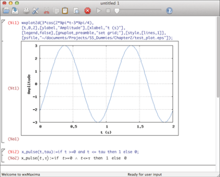
Figure 1-10: The wxMaxima notebook interface to Maxima.

You can send Maxima plots to a file in a variety of formats or display them directly in the notebook, as shown in Figure 1-11.

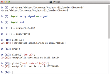
Figure 1-11: The IPython QT console window.

You can write and debug functions right from the console window, as shown in Figure 1-12.

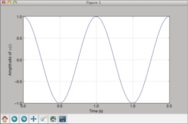
Figure 1-12: matplotlib plot window resulting from a call to plot(x,y) in IPython.

You can manipulate plots by using the controls you see at the bottom of the figure window. Plot cursors are also available. You can save plots from the command line or from the figure window. Many of the plots found in this book were created with matplotlib.

Seeing the Big Picture

Figure 1-13 illustrates the content organization of this book as an unfolding of core topics, starting from the time domain and moving to the frequency domain before exploring the s- and z-domains. Continuous (left side) and discrete (right side) signals and systems topics parallel each other every step of the way — with some continuous- and discrete-time topics shared (center) within a few chapters. The last four chapters, which follow the z-domain chapter, emphasize applications, including signal processing, wireless communications, and control systems.

I start with the time domain because this is where signals originate and where systems operate on signals (with the exception of transform domain processing, which is covered in Chapter 12). The frequency domain augments a base knowledge of both signals and systems and is important to grasping sampling theory, which leads to the processing of continuous-time signals in the discrete-time domain. The s- and z-domain are the last of the core topics, but by no means are they any less important than the topics that come before them. The s- and z-domains are particularly powerful when working with linear time-invariant systems described by differential and difference equations.

After covering the core topics, you can appreciate the chapter that focuses on how to work across domains (Chapter 15). Get a taste of how signals and systems fit into the real world of electrical engineering by reading the case studies at www.dummies.com/extras/signalsandsystems. Take a look at the application examples to get inspired when you're struggling to see the forest for the trees of the dense study of signals and systems.

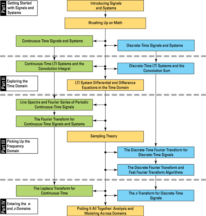
Figure 1-13: Signals and systems topic flow.