Chapter 11

The Discrete-Time Fourier Transform for ­Discrete-Time Signals

In This Chapter

Checking out the Fourier transform of sequences

Getting familiar with the characteristics and properties specific to the DTFT

Working with LTI system relationships in the frequency domain

Using the convolution theorem

If you’re hoping to find out how the discrete-time Fourier transform (DTFT) operates on discrete-time signals and systems to produce spectra and frequency response representations with units of radians/sample, you’re in the right place! And I hope it wasn’t too hard to find; Fourier theory is covered in four different chapters.

The Fourier transform (FT) (explored in Chapter 9) has the same capabilities as the DTFT, but it applies to the continuous-time cousins in the lands of continuous frequency. If you’re looking for a Fourier transform that’s discrete in both time and frequency, you need the discrete Fourier transform (DFT), which is the subject of Chapter 12. The Fourier series (covered in Chapter 8) applies to continuous-time periodic signals with a discrete frequency-domain representation.

Trig functions are integral to all forms of Fourier theory. In signals and systems, the trig functions are usually hidden inside a complex exponential, but Euler’s formula (see Chapter 2) tells you that a complex sinusoid is composed of a cosine on the real axis and a sine on the imaginary axis.

In terms of the DTFT, the forward transform (which moves a signal from the time to frequency domain) requires a summation; the inverse discrete-time Fourier transform (IDTFT) (which takes a signal from the frequency domain back to the world of time) requires an integral. This asymmetry may be unexpected if you’ve worked only with the continuous-time Fourier transform. But the DTFT produces a spectral function of a continuous frequency variable from a discrete-time signal or sequence.

The forward transform takes a discrete-time signal (sequence) as input, so a sum is required (not an integral, as in the continuous-time case). Inverse transforming requires integration over the frequency variable to return to the discrete-time domain. As a bonus, the summation of the forward transform often involves only the use of the geometric series (see Chapter 2).

The DTFT has properties and theorems that are similar to the Fourier transform (FT). But, unlike the FT, the DTFT spectrum is a periodic function of the frequency variable, which may seem rudimentary if you’re familiar with sampling theory (Chapter 10). Like the FT, the DTFT is a complex function of frequency, so magnitude and phase spectra appear.

In this chapter, I formally define the frequency response of linear time-­invariant (LTI) systems. (Check out Chapter 7 for a peek at the frequency response for linear constant coefficient difference equations.) I also show you the full utility of the frequency response by using the convolution theorem for the DTFT.

Getting to Know DTFT

In this section, I define the DTFT and IDFT and point out when these tools apply to specific types of signals and systems work. I also cover basic DTFT properties for both signals and systems and show you the mathematical link between the spectrum of a continuous-time signal and the spectrum of the corresponding discrete-time signal via uniform sampling. My intent is to show you how nicely the frequency-domain view of sampling theory from Chapter 10 fits with the spectrum of a discrete-time signal and to help you get comfortable working with the DTFT/IDFT.

The DTFT of sequence x[n] is defined by this summation:

Here, is the discrete-time frequency variable. The quantity is the signal spectrum of . The synthesis formula for getting from is the IDTFT equation:

The integration can be performed over any interval. Formally, the DTFT exists if is absolutely summable, meaning

Explore signals that violate this condition in the section “The DTFT of Special Signals,” later in this chapter.

Example 11-1: Find the DTFT of the exponential sequence . As a cautious first step, find out what conditions on a ensure that x[n] is absolutely summable. Next, find and then follow these steps:

1. Compute the absolute sum of by using infinite geometric series results from Chapter 2:

This first step reveals that the DTFT of exists only for .

2. Find the DTFT, which involves similar series-manipulation skills:

As expected, is a complex quantity. You now have your first DTFT transform pair:

Not too bad! Hold on to your geometric series skills for calculating the DTFT sum throughout this chapter.

Checking out DTFT properties

When discrete-time signals are real, some useful symmetry properties fall into place in the frequency domain. Parallel results exist for the Fourier series of Chapter 8 and the Fourier transform of Chapter 10, but when you’re working with a periodic spectrum for the DTFT, results are a bit different.

In general, the DTFT of is a complex function of , so viewing it in polar form (magnitude and angle) is convenient:

is the magnitude or amplitude spectrum, which parallels for the FT.

is the phase spectrum, which parallels for the FT.

The fact that the frequency variable always appears wrapped inside a complex exponential, such as , means that is periodic, with period . Why? Note that because .

The periodicity of the discrete-time spectrum is in sharp contrast to the FT, because the spectrum of a sampled continuous-time signal is repeated at multiples of the sampling rate (see Chapter 10). For a discrete-time signal, the sampling period is pretty much once per integer, meaning the sampling rate in radians per sample is . This justifies using any interval in the IDTFT integral.

For LTI systems, the frequency response is the DTFT of the impulse response, . So returning to the impulse response is just a matter of taking the IDTFT of . Find more on the impulse response and frequency response in the section “LTI Systems in the Frequency Domain,” later in this chapter.

Relating the continuous-time spectrum to the discrete-time spectrum

Among the differences between the Fourier transform for discrete-time signals and the Fourier transform for continuous-time signals are the nature of sequences and the connection to uniform sampling a continuous-time signal. In practice, you frequently find the sequence values by uniform sampling of the continuous-time signal . An impulse train with amplitude weights, the sample values represent this sampled continuous-time waveform:

The FT of is , where is the FT of , and . Now, relate to and ultimately .

Here’s a three-step process for developing the to relationship:

1. Find .

You can use the FT pair and the linearity theorem to get a term-by-term solution:

Notice that looks very much like the definition of the DTFT of x[n], except appears instead of .

2. Take the expression for from Step 1 and substitute to relate to :

3. Pair the results of Step 2 with the FT of the sampled continuous-time signal , as developed in Chapter 9:

where in the last line, is the FT of , using the based FT.

For x(t) bandlimited to fs/2 — or for , for — X(f ) is the FT of x(t). This result is significant because it links the frequency domain to continuous- and discrete-time systems, and it tells you — via the frequency axis mapping of f in hertz to in radians/sample () — exactly how the continuous-time spectrum becomes the corresponding discrete-time spectrum.

When you use ideal reconstruction (see Chapter 10) to convert y[n] back to y(t), a similar result holds: , where and . The reverse frequency axis mapping to f is .

In Chapter 15, I apply the relationship between the continuous- and discrete-time spectrums for modeling across domains. The time-domain connection is simply .

Getting even (or odd) symmetry ­properties for real signals

A real signal may be an even or odd function, and these conditions leave their mark in the frequency domain.

For , a real sequence, the spectrum is conjugate symmetric, which means that . To demonstrate this property, I work from the DTFT definition:

I rely on the fact that and .

Here are the important consequences of conjugate symmetry:

is even in , which implies that .

is odd in , which implies that .

is even in , which implies that .

is odd in , which implies that .

These observations also point out that is unique on a length interval, such as . Consider over one period spanning . Conjugate symmetry tells you that on the interval is on the interval . So given on the interval, you can extend to the .

From the periodicity of , you can replicate any other length interval knowing on the interval. Again, from periodicity, knowing any length interval is sufficient.

If is an even sequence (), it can be shown that is real, or . Similarly, if is an odd sequence (), it can be shown that is imaginary, or . (Find details on even and odd functions in Chapter 3.)

---

---

Example 11-2: Plot the spectra of for and comment on the observed symmetry properties. Example 11-1 reveals that .

You can use Python and Pylab to make the plots. Figure 11-1 shows plots of the real, imaginary, magnitude, and phase for .

In [101]: w = arange(-pi,pi,pi/500.)

In [102]: X = 1/(1 - 0.8*exp(-1j*w))

In [105]: plot(w,real(X))

In [110]: plot(w,imag(X))

In [115]: plot(w,abs(X))

In [121]: plot(w,angle(X))

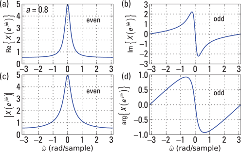
Figure 11-1: The spectrum of 0.8nu[n] in terms of the real (a), imaginary (b), magnitude (c), and phase (d).

The conjugate symmetry of is visible in Figure 11-1 in both the rectangular and polar forms. Because is neither even nor odd, contains both real and imaginary parts.

Example 11-3: Find the DTFT of the even sequence . From the start, you may be thinking that a two-sided exponential should be only twice as hard as the one-sided exponential anu[n]. Here, you can find out.

There are four steps to solving this problem:

1. To successfully tackle a signal with an absolute value, break it into two pieces.

The convenient split point here is between n = –1 and n = 0. The DTFT of x[n] is the sum of the DTFT of each piece:

2. In the first sum, S1, change variables (let m = –n) so the sum runs from 1 to , and then re-index the sum to start at 0 and subtract 1, which is what the m = 0 term contributes:

3. Evaluate the second sum, S2, by noting that it’s already in standard infinite geometric series form (also see Example 11-1):

4. Combine the terms over a common denominator:

This last step is optional, but the final form is compact and clean.

As a check on the hand calculations, you can use a CAS like Maxima:

This calculation reveals (line 3) and is a great help when you’re trying to get comfortable with geometric series manipulation. Getting to the final form takes some finessing with the simplifying rules in Maxima. Notice that is indeed real, because the signal is real and even.

Example 11-4: Find the DTFT of the odd sequence .

For short finite-length sequences, transforming term by term is best. Expand out the definition and include only the terms corresponding to nonzero values of x[n]:

Here, the only terms you need to include are n = –2, –1, 1, and 2. Simplify by using Euler’s formula for sine:

For odd, is pure imaginary.

Studying transform theorems and pairs

Think of a DTFT theorem as a general purpose transform pair — or a catalog of frequency spectra corresponding to specific discrete-time signals — because a theorem considers the DTFT of one or more generic signals under some transformation, such as convolution. By taking full advantage of theorems and pairs, you can get fast and efficient in solving problems.

In this section, I provide tabular listings of DTFT theorems and pairs. I also provide short proofs of the most popular theorems and develop a couple of transform pairs.

Figure 11-2 offers a catalog of useful DTFT theorems.

These DTFT theorems are similar to the FT theorems in Chapter 9:

Linearity: .

The proof follows from the definition and the linearity of the sum ­operator itself.

Time shift: .

To prove, I start from the definition but change variables :

Frequency shift: .

Using the DTFT definition,

Convolution: The convolution of two sequences (see Chapter 6) is defined as .

It can be shown that convolving two sequences is equivalent to multiplying the respective DTFTs: .

Figure 11-2: Useful DTFT theorems.

A table of DTFT pairs (provided in Figure 11-3) is invaluable when you work problems. Unless you’re required to prove a particular pair, I see no sense in starting a problem empty-handed.

Figure 11-3: Useful DTFT pairs.

Here are a couple of transform pairs that you’ll likely use when studying signals and systems.

Impulse sequence: .

This pair comes from the definition from the sifting property of the impulse sequence.

Rectangular pulse (window) sequence: The rectangular pulse or window sequence is defined as

You can find the DTFT by direct evaluation, recognizing that the sum is a finite geometric series and factoring to form a ratio of sine functions:

The pair is .

Example 11-5: If , find . The brute-force approach (plugging directly into the DTFT definition) works, but I recommend taking advantage of theorems and transform pairs to streamline your work:

1. Rewrite in a form that anticipates the use of certain theorems:

2. Apply the time shift theorem (Line 2 in Figure 11-2):

3. Apply transform pair, Line 3 in Figure 11-3, assuming :

Working with Special Signals

Some signals aren’t absolutely summable, but you can find a meaningful DTFT for them. (I explore this kind of situation in Chapter 9, too, by using Fourier transforms in the limit to allow impulse functions in the frequency domain.) In this section, I describe mean-square convergence and Fourier transforms in the limit for the DTFT. By using mean-square convergence, I develop a transform pair for an ideal low-pass filter. Fourier transforms in the limit allow impulse functions in the frequency domain.

Getting mean-square convergence

A form of convergence that’s weaker than absolute convergence is known as mean-square convergence, which requires square summability of x[n]:

This condition is easier to satisfy than absolute summability; but with mean-square convergence, the DTFT may not converge pointwise in the frequency domain. (Chapter 8 explores the trouble with getting the Fourier series of a square wave to converge.)

A rectangular or low-pass spectrum is defined on the fundamental interval to be

where is the spectrum bandwidth in rad/sample.

Here, I’m talking about a signal spectrum, but this definition also applies to the frequency response of an ideal low-pass filter. Being able to synthesize an ideal low-pass filter allows you to separate a desirable signal from an undesirable one, even when they’re right next to each other spectrally.

Given the spectrum, you can work backward to get the signal by using the IDTFT:

A rectangle in the frequency domain is a sampled sinc function in the time domain (find the continuous-time version in Chapter 9).

In Figure 11-4, I plot for over the interval to show how quickly the sinc function decays to 0 and to point out how important the small tail values are in the frequency domain when considering truncation.

The absolute sum of this sequence diverges because the terms are of the form , which is the harmonic series, and known to diverge. The sum of converges so is square summable.

It would be nice if I could form a term approximation to and arrive at a likeable approximation to the ideal low-pass spectrum (read: filter), too. Luckily, I can! The approximation to the spectrum/frequency response takes the form

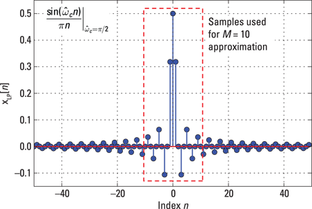
Figure 11-4: A plot of for .

For the case of a filter, this means you can use a 2M + 1-tap finite impulse response (FIR) filter to approximate an ideal low-pass filter. But to make the filter causal, you also need a time delay of M samples to the right. Your intuition may say that by increasing M, the filter approximation gets better — and it does get better in the sense of being more rectangular shaped (like the ideal rectangular spectrum definition) — but the ripples on both sides of remain fixed in amplitude.

I use Python to check by writing a loop inside the IPython environment to numerically calculate the spectrum and then plot results (see Figure 11-5).

In [138]: w = arange(0,pi,pi/500.)

In [139]: X_LP = zeros(len(w))+1j*zeros(len(w))

In [140]: for n in range(-10,10+1):

     ...: X_LP += pi/2./pi*sinc(pi/2.*n/pi)*exp(-1j*w*n)

     ...:

In [140]: plot(w,20*log10(abs(X_LP)))

This exercise reveals that at the band edges, where the spectrum transitions from 1 to 0, quite a bit of ringing occurs. The peak passband (0 dB spectrum level) ripple is 0.75 dB, and the peak side lobe level is only 21 dB below the passband; both values are independent of M! The passband to stopband transition occurs faster (narrower band of frequencies) as M increases, so your intuition is partially confirmed. The ripple isn’t good.

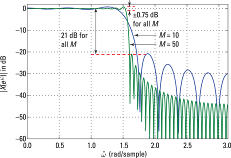
Figure 11-5: A term approximation to an ideal low-pass magnitude spectrum for M = 10 and 50.

Window functions to the rescue. To reduce the ripple level, you can employ window functions (described in Chapter 4). With windowing, you multiply the truncated sinc function signal by a nonconstant shaping function, w[n], which smoothly transitions from 1 to 0 at the window edges. The DTFT of the smooth w[n] has a much smaller ripple level, and passes that on to the overall spectrum of x[n]w[n]. The ripple level is made small at the expense of a wider transition frequency band. You can, however, narrow the transition band by increasing M. This story does indeed have a happy ending.

Finding Fourier transforms in the limit

The Fourier transform in the limit approach allows impulse functions to exist in the frequency domain. As a specific case, suppose you have a sequence , which has DTFT for . Because is always periodic, the complete representation is

The spectrum in the discrete-time domain is always periodic with period . When a spectrum involves impulse functions as opposed to a function of , the periodicity isn’t automatic, so you need the doubly infinite sum. Don’t let this apparent complexity confuse you. For , the only impulse function is .

To find , operate with the IDTFT , which establishes the following DTFT pair (through the sifting property of the impulse function):

If , then is just a constant, so .

Now, suppose . Using Euler’s formula for cosine, find that

See the spectrum of in Figure 11-6.

Figure 11-6: The spectrum of .

Example 11-6: Say a continuous-time sinusoid is sampled over a finite time interval to produce the discrete-time signal , where is a rectangular ­windowing function corresponding to the capture interval. The signal, both continuous-time and discrete-time, before and after windowing, is plotted in Figure 11-7.

A transform pair and transform theorem make short work of this problem.

1. Use the transform pair from Line 6 of Figure 11-3:

2. To get , use the multiplication, or windowing, theorem (Line 5 from Figure 11-2).

In the end, the calculation requires a convolution in the frequency domain between and :

Figure 11-7: The windowed sequence x[n] (stems) and the underlying continuous-time sinusoid (dashed).

Step 2 appears messy, but only one pair of the cosine impulse functions lies on the interval that you integrate over. And the integration itself is straightforward because the impulse function just sifts out the integrand sampled at .

I plot the spectrum of the windowed cosine in Figure 11-8, using Python. I compute the DTFT with the function freqz() from the SciPy module signal.

In [206]: n = arange(0,10)

In [207]: x = cos(3*pi/4.*n)

In [208]: w = arange(-pi,pi,pi/500.)

In [209]: w_in = arange(-pi,pi,pi/500.)

In [210]: w,X = signal.freqz(x,1,w_in)

In [211]: plot(w,abs(X))

Impressed? Only ten samples of the cosine signal results in the spectral blobs at . Not too bad, but this is a far cry from impulse functions, which is what you’d see if the windowing wasn’t present.

I increased M to 50 to show how much improvement a five-times the window length provides. In the end, M must be large enough to provide a reasonable estimate of the sinusoid parameters A and . As M increases the spectrum of the window, , gets narrower, because the spectrum width is proportional to 1/M. When the window spectrum is convolved with the frequency domain impulse functions of the sinusoid, the result is a more compact spectrum shape. Find a more detailed example of spectral estimation using windows online at www.dummies.com/extras/signalsandsystems.

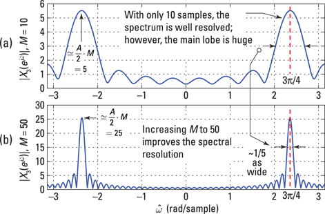
Figure 11-8: The spectrum of a windowed cosine, using (a) and (b).

LTI Systems in the Frequency Domain

For LTI systems in the time domain (see Chapter 6), a fundamental result is that the output, , is the input, , convolved with the system impulse response, : .

To carry this result to the frequency domain, simply take the DTFT of both sides:

This is the convolution theorem for the DTFT.

The quantity is known as the transfer function or frequency response of the system having impulse response . This is a special FT. If you want to get via multiplication in the frequency domain, you just need to compute the inverse DTFT of the product: .

You can write this input/output relationship as the ratio of the output spectrum to the input spectrum, . If , then , and the output spectrum takes its shape entirely from because .

Considering the properties of the frequency response, keep in mind that for real, .

Also, the output energy spectral density is related to the input energy spectral density and the frequency response because the convolution theorem says :

As a result of the FT convolution theorem, you can develop the cascade relationship from the block diagram of Figure 11-9. (See Chapter 5 for cascading LTI systems in the time domain.)

Figure 11-9: Cascade of LTI systems in the frequency domain.

In the frequency domain, and so, upon linking the two equations, you have the following:

As a result of the FT convolution theorem, you can develop the parallel connection relationship from the block diagram of Figure 11-10.

Figure 11-10: Parallel connection of LTI systems in the frequency domain.

In the frequency domain, the following is true:

So

Taking Advantage of the Convolution Theorem

By working in the frequency domain, you can avoid the tedious details of the convolution integral (covered in Chapter 6). In particular, you can find time-domain signals at the output of a system by multiplying the input spectrum with the frequency response and then using the inverse transform to return to the time domain. The output you seek may be in response to an impulse or a step or a very specialized signal, and along the way, you may be interested in the output spectrum, too.

Example 11-7: Use the DTFT to determine both the impulse response and frequency response directly from a linear constant coefficient (LCC) difference equation. Consider the following:

Find and . The problem solution breaks down into four steps:

1. Take the DTFT of both sides of the difference equation, using the time shift theorem (Line 2 of Figure 11-2):

Because , .

2. Solve for by using simple algebra on the results of Step 1:

3. To get , use the inverse transform by breaking the expression into two terms:

4. Use transform pair Line 3 in Figure 11-3 on both terms and use the time shift theorem on the second term:

The time shift factor replaces n in all locations where it occurs in the second term.