Chapter 3

Continuous-Time Signals and Systems

In This Chapter

Defining signal types

Classifying specific signals

Modifying signals

Looking at linear and time-invariant systems

Checking out a real-world example system

In signals and systems, the distinction continuous time refers to the independent variable, time t, being continuous (see Chapter 1). In this chapter, I provide an inventory of signal types and classifications that relate to electrical engineering and cover the process of figuring out the proper description for a particular signal. Like their discrete-time counterparts described in Chapter 4, continuous-time signals may be classified as deterministic or random, periodic or aperiodic, power or energy, and even or odd. Signals hold multiple classifications.

Also in this chapter, I describe the process of moving signals around on the time axis. Modeling the placement of signals on the time axis affects system functionality and relates to the convolution operation that’s described in Chapter 5. Time alignment of signals entering and leaving a system is akin to composing a piece of music.

Don't worry; I include a drill down on system types and classifications here, too, focusing on five property definitions: linear, time-invariant, causal, memoryless, and stability. Find a system-level look at the signals and systems model of a karaoke machine at www.dummies.com/extras/signalsandsystems. The signal flow through this system consists of two paths: one for the recorded music and the other for the singer's voice that enters the microphone. The subsystems of the karaoke machine act upon the two input signal types — in this case, both random signals — to finally end up at the speakers, which convert the electrical signals to sound pressure waves that your ears can interpret.

Considering Signal Types

Knowing the different types of signals makes it possible for you to provide appropriate stimuli for the systems in your product designs and to characterize the environment in which a system must operate. Both desired and undesired signals are present in a typical system, and models make it easier to create products that can operate in a range of different conditions.

Some signals types are a means to the end — the signal is designed to fulfill a purpose, such as carrying information without wires. Other signal types are useful for characterizing system performance during the design phase. Still other signal types are intended to make things happen in an orderly fashion, such as timing events while a person arms and disarms a burglar alarm.

Signal types described in this section include sinusoids, exponentials, and various singularity signals, such as step, impulse, rectangle pulse, and triangle pulse. Real signals are typically composed of one or more signal types.

Exponential and sinusoidal signals

In this section, I introduce you to two of the most fundamental and important signal types:

Complex exponential: This signal occurs naturally as the response (output) of linear time-invariant systems (see the section “Checking Out System Properties,” later in this chapter) to arbitrary inputs.

Real and complex sinusoids: These signals function inside electronic devices, such as wireless communications, and form the basis for the Fourier analysis (frequency spectra), which is described in Part III of this book.

A general complex exponential signal, which also includes exponentials and real complex sinusoidal signals, is , where, in general, and . This is a lot to handle when you think about it. The signal contains two parameters but, because each parameter is generally complex — having a real and imaginary part (for ) or magnitude and phase (for ) — four parameters are associated with this signal. To make this concept manageable to study, I break down the signal into several special cases and discuss them in the following sections.

Real exponential

For real, () and , meaning . You arrive at the real exponential signal . Of the two parameters that remain, A controls the amplitude of the exponential and controls the decay rate of the signal.

In practice, the real exponential signal also contains the function u(t), known as the unit step function (see the later section “Unit step function” for details). For now, all you need to know about the step function is that it acts as a switch for a function of time. The switch u(t) is 0 for t < 0 and 1 for t > 0. Using u(t), limit x(t) to turning on at by writing .

Example 3-1: To plot the real exponential signal for various values of , use Python with PyLab. See the results in Figure 3-1.

In [689]: t = arange(-2,10,.01)

In [690]: plot(t,2*exp(-.2*t)*ssd.step(t))

In [691]: plot(t,2*exp(0*t)*ssd.step(t),'b--')

In [692]: plot(t,2*exp(.2*t)*ssd.step(t),'b-.')

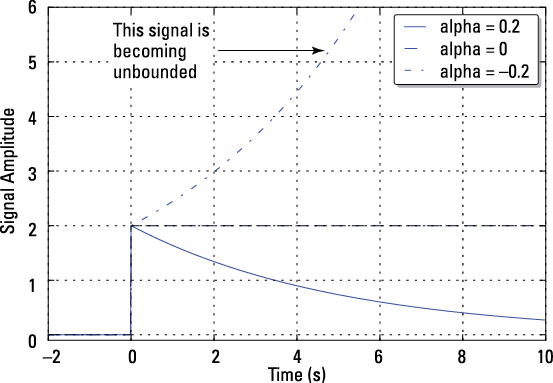
Figure 3-1: A real exponential signal for positive, zero, and negative.

Complex and real sinusoids

For imaginary () and complex (), the signal becomes a complex sinusoid with real and imaginary parts being the cosine and sine signal, respectively. Take a closer look:

The last line comes from applying Euler’s formula.

By breaking out the real and imaginary parts as , you get the real cosine and sine signals: and . In this signal model, A is the signal amplitude, is the signal frequency in rad/s or when using the substitution , f­0 is the frequency in hertz (cycles per second), and is the phase. See the later section “Deterministic and random” for more information on these parameters.

The real cosine signal is one of the most frequently used signal models in all of signals and systems. When you key in a phone call, you’re using (and hearing) a combination of two sinusoidal signals to dial the phone number. The wireless LAN system you use at work or home also relies on the real sinusoid signal and the complex sinusoid. A real sinusoid signal with rad/s is the signal that enters your home to deliver energy (power) to run your appliances and lights. Modern life is filled with the power of the sinusoidal signal.

The case of K real sinusoids is also useful in general signal processing and communications applications. You simply add together the sinusoidal signals:

, with the substitution

This model can represent the result of pressing one or more keys on a piano keyboard.

Damped complex and real sinusoids

As a special case of the general complex exponential, assume that is complex , is complex, and u(t) is included, so the signal turns on for . The signal becomes a damped complex sinusoid with real and imaginary parts being damped cosine and sine signals, respectively:

The term damped means that drives the signal amplitude to 0 as t becomes large. The sinusoid sine or cosine is the other time-varying component of the signal. Breaking out the real and imaginary parts,

Have you ever experienced a damped sinusoid? Physical examples include a non-ideal swinging pendulum or your car’s suspension after you hit a pothole. In both cases, the oscillations eventually stop due to friction. With an appropriate measuring device, the physical motion can convert to an electrical signal. In the car example, the signal may be fed into an active ride control system and other inputs to modify the suspension system.

Singularity and other special signal types

As preposterous as it may sound, sinusoidal signals don’t rule the world. You need singularity signals to model other important signal scenarios, but this type of signal is only piecewise continuous, meaning a signal that has a distinct mathematical description over contiguous-time intervals spanning the entire time axis . The piecewise character means that a formal derivative doesn’t exist everywhere. A singularity signal may also contain jumps.

In this section, I describe a few of the most common singularity functions, including rectangle pulse, triangle pulse, unit impulse, and unit step. With these functions, you can put together many special waveforms, such as the one shown in Figure 3-8, later in this chapter.

Rectangle and triangle pulse

Two useful singularity signal types used in signals and systems analysis and modeling are the rectangle pulse, , and triangle pulse, .

Here’s the piecewise definition of the rectangle pulse:

This signal contains a jump up and a jump down. Note: Otherwise is math terminology for all the remaining time intervals on not specified in the definition. For the rectangle pulse, that would be . And also assume that τ is positive.

Here is the definition for the triangle pulse:

See plots of these two pulse signals in Figure 3-2.

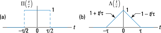
Figure 3-2: The rectangle pulse (a) and the triangle pulse (b).

The full base width of the rectangle pulse is ; for the triangle pulse, it’s . This is no accident. Check out Chapter 5 to find out how to get a triangle pulse of base width by convolving two rectangle pulses with a width of .

Here are the Python functions for these two signal types:

def rect(t,tau):

x = np.zeros(len(t))

for k,tk in enumerate(t):

if np.abs(tk) > tau/2.:

x[k] = 0

else:

x[k] = 1

return x

def tri(t,tau):

x = np.zeros(len(t))

for k,tk in enumerate(t):

if np.abs(tk) > tau/1.:

x[k] = 0

else:

x[k] = 1 - np.abs(tk)/tau

return x

The functions are designed to accept ndarray variables when using PyLab. Later, in Figure 3-8, these functions create a quiz problem. Note that I use Maxima for computer algebra–oriented calculations. For numerical calculations, particularly those that benefit from working with arrays or vectors, I use Python.

Unit impulse

You use the unit impulse, or Dirac delta function signal type, as a test waveform to find the impulse response of systems in Chapter 4. It’s a fundamental but rather mysterious signal.

---

---

You can define this signal only in an operational sense, meaning how it behaves. The signal appears as a spike, but the spike has zero width and unity area. This is confusing at first. But think of the cue ball striking another ball in a game of billiards. The momentum transfers instantly (impulsively), and the struck ball begins to roll. In an electrical circuit, think of a battery momentarily (very momentarily) making contact with the circuit input terminals. The circuit responds with its impulse response.

Operationally, the delta function has the following key properties:

The signal appears as a function with unit area located at . You can sift out a single value of the function x(t), which is assumed to be continuous at , by bringing it inside the integral:

This result is known as the sifting property of the unit impulse function. To actually put your hands on something that closely resembles the true unit impulse function, define the test function :

Notice that this function has unit area, like , and is focused at t = 0. In fact, as desired, the signal behaves like as , or . To illustrate the action of the sifting property, I first sketch the integrand by using in Figure 3-3a and then using in Figure 3-3b.

The proper way of plotting is to draw it as a vertical line with an arrow at the top. The location on the axis is where the argument is 0, as in , and height corresponds to the area. That means has location t = 0 and a height of 1, and has location and height A. See this in Figure 3-3b.

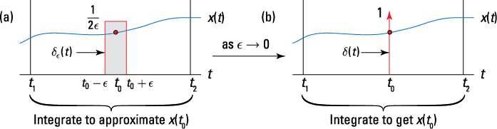
Figure 3-3: A graphical depiction of the sifting property, using (a) and then (b).

Unit step function

The unit step function, u(t), is also a singularity function. A popular use is modeling signals with on and off gates. In Chapter 5, I describe the step response of a system. Start from the unit impulse:

Thinking of , you can say . In the limit, u(t) contains a jump at t = 0, so it’s not defined.

You can program the unit step in Python:

def step(t):

x = np.zeros(len(t))

for k,tt in enumerate(t):

if tt >= 0: # the jump occurs at t = 0

x[k] = 1.0

return x

---

---

The step function is also available in ssd.py. To return to unit impulse function, just differentiate u(t) to get

Don’t sweat the details about the existence of the derivative at t = 0. Just replace the derivative at the discontinuity with a unit impulse function of height equal to the jump height. Note that this appears to violate what you probably learned in calculus about derivatives, but the unit impulse function fits perfectly in an engineering math sense.

Example 3-2: To practice working with the derivatives of signals that incorporate singularity functions, consider the derivative of the rectangle and triangle pulse functions.

The derivative of contains two unit impulse functions because it contains two jumps. A jump by 1 at , and a jump down by 1 at :

The derivative of doesn’t contain jumps, but it does contain three points of discontinuity, . When taking the derivative, focus on the derivative away from these points:

Figure 3-4 shows both signal derivatives.

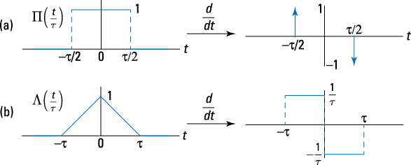
Figure 3-4: Derivatives of (a) and (b).

Getting Hip to Signal Classifications

Signals are classified in a number of ways based on properties that the signals possess. In this section, I describe the major classifications and point out how to verify and classify a given signal. Classifications aren’t mutually exclusive. A periodic signal, for example, is usually a power signal, too. And a signal may be even and aperiodic.

Deterministic and random

A signal is classified as deterministic if it’s a completely specified function of time. A good example of a deterministic signal is a signal composed of a single sinusoid, such as with being the signal parameters. A is the amplitude, is the frequency (oscillation rate) in cycles per second (or hertz), and is the phase in radians. Depending on your background, you may be more familiar with radian frequency, , which has units of radians/sample. In any case, x(t) is deterministic because the signal parameters are constants.

Hertz (Hz) represents the cycles per second unit of measurement in honor of Heinrich Hertz, who first demonstrated the existence of radio waves.

A signal is classified as random if it takes on values by chance according to some probabilistic model. You can extend the deterministic sinusoid model to a random model by making one ore more of the parameters random. By introducing random parameters, you can more realistically model real-world signals.

To see how a random signal can be constructed, write , where corresponds to the drawing of a particular set of values from a set of possible outcomes. Relax; incorporating random parameters in your signal models is a topic left to more advanced courses. I simply want you to know they exist because you may bump into them at some point.

To visualize the concepts in this section, including randomness, you can use the IPython environment with PyLab to create a plot of deterministic and random waveform examples:

In [234]: t = linspace(0,5,200)

In [235]: x1 = 1.5*cos(2*pi*1*t + pi/3)

In [237]: plot(t,x1)

In [242]: for k in range(0,5): # loop with k=0,1,…,4

     ...: x2 = (1.5+rand(1)-0.5))*cos(2*pi*1*t + pi/2*rand(1)) # rand()= is uniform on (0,1)

     ...: plot(t,x2,'b')

     ...:

See the results in Figure 3-5, which uses a PyLab subplot to stack plots.

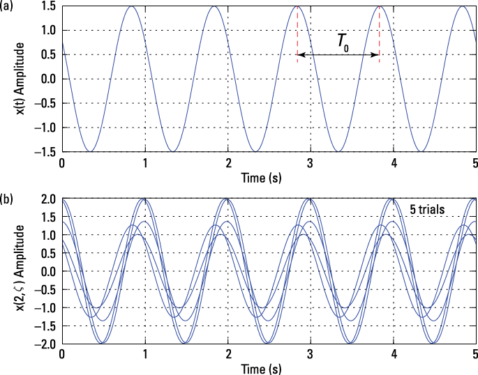
Figure 3-5: A deterministic sinusoid signal (a) and an ensemble of five random amplitude and phase sinusoids (b).

Generate the deterministic sinusoid by creating a vector of time samples, t, running from zero to five seconds. To create the signal, x1 in this case, I chose values for the waveform parameters .

For the random signal case, A is nominally 1.5, but I added a random number uniform over (–0.5, 0.5) to A, making the composite sinusoid amplitude random. The frequency is fixed at 1.0, and the phase is uniform over . I create five realizations of using a for loop.

Periodic and aperiodic

Another type of signal classification is periodic versus aperiodic. A signal is periodic if , where , the period, is the largest value satisfying the equality. If a signal isn’t periodic, it’s aperiodic.

When checking for periodicity, you’re checking in a graphical sense to see whether you can copy a period from the center of the waveform, shift it left or right by an integer multiple of , and if it perfectly matches the signal T0 seconds away. The single sinusoid signal is always periodic, and the proof, which relies on simple trigonometry (flip to Chapter 2 for a trig refresher), allows you to determine what the period is.

Example 3-3: To establish that a single sinusoid signal is periodic and to determine the period, follow these steps:

1. Ask yourself: What does it take to make the equality hold?

Making the arguments equal seems to be the only option.

2. Expand the argument of the cosine on the right side to see the impact of the added :

Cosine is a modulo function; that is, the functional values it produces don’t change when the argument is shifted by integer multiples of , which makes the single sinusoid a periodic signal from the get-go.

3. To establish the period, observe that forcing means .

Because is the fundamental period, is the fundamental frequency; they’re reciprocals.

Example 3-4: Figure 3-6a shows a periodic signal known as a periodic pulse train because it has an infinite train of pulses. Each pulse has width , and the ellipsis indicate that the pulse train continues in both directions. The pulses that follow each other don’t have to be periodic, though. In Figure 3-6b, a waveform with a single isolated pulse or just a few pulses makes the signal aperiodic.

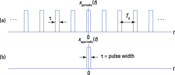
Figure 3-6: A periodic pulse train signal with pulse width and period (a) and a single, aperiodic pulse (b).

Considering power and energy

To classify a signal x(t) according to its power and energy properties, you need to determine whether the energy is finite or infinite and whether the power is zero, finite, or infinite. The measurement unit for power and energy are watts (W) and joules (J).

In circuit theory, watts delivered to a resistor of R ohms is represented as

, where V is voltage in volts and I is current in amps.

Figure 3-7 shows that a circuit is composed of resistor and voltage sources, demonstrating the interconnection of signals and systems with physics and circuit concepts. A simple power calculation in circuit analysis becomes instantaneous power with time dependence, and the resistance is normalized to 1 ohm as used in signals and systems terminology.

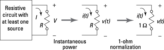
Figure 3-7: Relating power in a circuit to signals and systems 1-ohm normalization.

With the circuit calculation of power, you can introduce time dependence and define a signal’s instantaneous power as

Computer and electrical engineers use the abstraction available through mathematics to work in a convenient 1-ohm environment.

The significance of the 1-ohm impedance normalization is that instantaneous power is simply or . It’s convenient then to use to represent the signal — voltage or current. Keep in mind that, unless told otherwise, in all signals. When modeling results need to be coupled to physical, real-world measurements, you can add back in the resistance, or impedance level.

Average power, P (watts), and average energy, E (joules), are defined as follows:

The is used when the signal happens to be complex. For x(t) periodic, you can simplify the average power formula to

where is the period. Note that the single limit on the far right integral means that you can use any interval for the calculation. The limit is gone, and the integration now covers just one period.

For x(t) to be a power signal, and . To understand why this is, think about a signal that has nonzero but finite power. Integrating the power over all time gives you energy. When you integrate nonzero finite power over infinite time, you get infinite energy.

An energy signal requires and . Yet some signals are neither power nor energy types because they have unbounded power and energy. For these, .

Mathematically, a signal can have infinite power, but that’s not a practical reality. Infinite energy indicates that the signal duration is likely infinite, so it doesn’t make sense to deal with energy. Power, on the other hand, is energy per unit time averaged over all time, making power more meaningful than energy.

---

---

Here are a few examples of power and energy calculations.

Example 3-5: To classify a signal with one or two cosines as a power or energy function, follow this process:

For a single real sinusoid , you can take advantage of the fact that x(t) is periodic with a period in these calculations:

This is a power signal because E is infinite and P is finite.

For a signal with two real sinusoids, such as , as long as , you can use this equation to solve for P:

This is the sum of powers for single sinusoids, which is all you need. Periodicity of x(t) isn’t a requirement.

Example 3-6: Consider a signal with two sinusoids:

Can this signal be periodic? The individual sinusoid periods are . For the composite signal to be periodic, must be commensurate, which means you seek the smallest values so that periods of duration are equal to periods of duration . Here’s how to set it up in an equation:

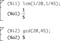
The ratio of the two periods and, likewise, the frequencies must be a rational number. The fundamental period is . In algebraic terms, you can state it as the least common multiple (LCM) of the periods or the greatest common divisor (GCD) of the frequencies:

If Hz and Hz, Hz, so .

If you have a calculator that incorporates a computer algebra system (CAS), you may be able to use the LCM and GCD functions to check your hand calculations. If not, consider using Maxima (see Chapter 1 for details).

The LCM and GCD functions in Maxima confirm the hand calculations presented earlier:

Periodicity among multiple sinusoids is essential to Fourier series (covered in Chapter 8).

Example 3-7: To classify as a power or energy (or neither) signal with respect to , consider the following three cases. To properly classify x(t), you need to find both the energy (E) and the power (P) values. Using the definition given in the section “Considering power and energy,” find out whether E is finite or infinite and whether P is zero, finite, or infinite.

Case 1:

This is an energy signal because E is finite and P is zero.

Case 2:

This is a power signal because E is infinite and P is finite.

Case 3: :

This signal is neither power nor energy because P is infinite. The signal amplitude becomes unbounded (refer to Figure 3-1). The term unbounded means magnitude approaching infinity.

Sinusoidal signals are power signals. For a single sinusoid, the power is just

. For K sinusoids at distinct frequencies, the signal power is .

If sinusoids have the same frequency, you need to combine these terms by using the phasor addition formula (described in Chapter 2). To figure out the power of each like frequency, you just need the equivalent amplitude.

Even and odd signals

Signals are sometimes classified by their symmetry along the time axis relative to the origin, t = 0. Even signals fold about t = 0, and odd signals fold about t = 0 but with a sign change. Simply put,

To check the even and odd signal classification, I use the Python rect() and tri() pulse functions to generate six aperiodic signals. Here's the code for generating two of the signals:

In [759]: t = arange(-5,5,.005) # time axis for plots

In [760]: x1 = ssd.rect(t+2.5,3)+ssd.rect(t-2.5,3)

In [763]: x4 = ssd.rect(t+3,2)-ssd.tri(t,1)

+ssd.rect(t-3,2)

Check out the six signals, including the classification, in Figure 3-8.

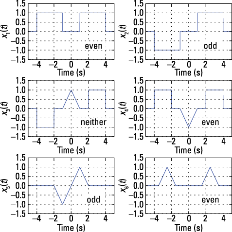
Figure 3-8: Six aperiodic waveforms that are classified as even, odd, or neither.

To discern even or odd, observe the waveform symmetry with respect to t = 0. Signals x1(t), x4(t), and x6(t) are even; they fold nicely about t = 0. Signals x2(t) and x5(t) fold about t = 0 but with odd symmetry because the waveform on the negative time axis has the opposite sign of the positive time axis signal. Signal x3(t) is neither even nor odd because a portion of the waveform, the triangle, is even about 0, while the rectangles are odd about 0. Taken in combination, the signals are neither even nor odd.

A single sinusoid in cosine form, without any phase shift, is even, because it’s symmetric with respect to t = 0, or rather it’s a mirror image of itself about t = 0. Mathematically, this is shown by the property of being an even signal:

Similarly, a single sinusoid in sine form, without any phase shift, is odd, because it has negative symmetry about t = 0. Instead of an exact mirror image of itself, values to the left of t = 0 are opposite in sign of the values to the right of t = 0. This is mathematically an odd signal:

If a nonzero phase shift is included, the even or odd properties are destroyed (except for ).

Transforming Simple Signals

Signal transformations, such as time shifting and signal flipping, occur as part of routine signal modeling and analysis. In this section, I cover these signal manipulation tasks as well as superimposing of signals to help you get more comfortable with these processes as they relate to continuous-time signals. (For details on these tasks for discrete-time signals, flip to Chapter 6.)

Time shifting

Time shifting signals is a practical matter. By design, signals arrive at a system at different times. A signal sent from a cellphone arrives at the base station after a time delay due to the distance between the transmitter and receiver. Mathematically, modeling this delay allows you, the designer, to consider the impact of time on system performance.

Given a signal x(t), consider , where may be positive, zero, or negative.

For the shifted or transformed sequence , x(0) occurs when , which implies that the signal is shifted by seconds. If is positive, the shift is to the right; if is negative, the shift is to the left. For the unshifted signal x(t), x(0) occurs when .

When working with the rectangle or triangle pulse function, think of moving the active region, or support interval, of the pulse. For example, the support interval of is . The shifted pulse has support interval . If you isolate t between the two inequalities by adding to both sides, then the support interval is . The support interval shifts by seconds. See Figure 3-9 for a graphical depiction of time-axis shifting.

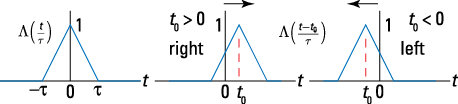
Figure 3-9: Time shifting depicted for the triangle pulse.

Flipping the time axis

Processing signals in the time domain by linear time-invariant systems requires a firm handle on the concept of flipping signals (see Chapter 5). Flipping, or time reversal, of the axis corresponds to . The term flipping describes this process well because the waveform literally flips over the point . Everything reverses. What was at is now located at , for example. You can apply this to all signals, including rectangular pulses, sinusoidal signals, or generic signals. Check out Figure 3-10 to see the concept of flipping for a generic pulse signal.

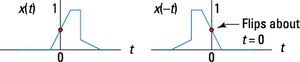
Figure 3-10: Axis flipping (reversing) for a generic pulse signal.

Putting it together: Shift and flip

Shifting and flipping a signal over the time axis corresponds to . Think of t in this axis transformation as the axis for plotting the signal and as a parameter you can vary. You can visualize the transformed signal as a two-step process.

1. Manipulate the signal argument so you can see the problem as shift and then flip: .

If, for a moment, you ignore the minus sign between the bracket and parentheses on the right, , it looks like x(t) is simply shifted to the right by (assume ).

2. Bring the minus sign back in, realizing that this flips the signal.

The minus sign surrounds , so the signal flips over the point .

Figure 3-11 shows a shifting and flipping operation.

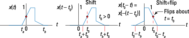
Figure 3-11: Combined signal transformation of shifting and flipping.

Confirm that the leading and trailing edges of x(t), denoted , respectively, transformed as expected. In the plot of , does the point correspond to the original leading edge ? To find out, plug into :

To check the trailing edge location, consider the time location of the far left side of the signal. The leading edge is at the far right side of the signal.

Flip to Chapter 5 for more information on shifting and flipping signals when working with the convolution integral.

Superimposing signals

Think about a time when you’ve been in a loud public space and can clearly hear the voice of the person to whom you’re talking; the other sounds register to you as background noise. The concept of superimposing signals is similar.

In mathematical terms, superimposing signals is a matter of signal addition:

Each component signal, , may actually be an amplitude that’s a scaled and time-shifted and/or flipped version of some waveform primitive.

The signals with multiple sinusoids described in the earlier section “Exponential and sinusoidal signals” represent superimposed signals, and the example signals in Figure 3-8 were generated by using time-shifted and added rectangle and triangle pulses. In real-world scenarios, you have environments that contain superimposed signals — whether by design or as a result of unwanted interference.

Example 3-8: Signal from Figure 3-8 is a sum of three pulse signals. I used the Python rect() and tri() pulse functions to create the signal, but I was thinking about this mathematical description when I created it:

This involves the use of signal time shifting and superposition. Note also that the Python code for generating the signal as a vector (actually a PyLab ndarray) of signal samples, x4, is an almost verbatim match with the mathematical equation for .

Checking Out System Properties

Generally, all continuous-time systems modify signals to benefit the objectives of an engineering design (see Chapter 1). Consider the system input/output block diagram of Figure 3-12. The input signal has fuzz on it, and the output is clean, suggesting that the system operator is acting as a fuzz-removing filter. Fuzz to you is noise to me.

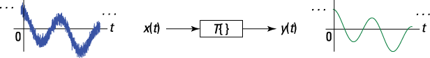
Figure 3-12: System input/output block diagram.

All systems have specific jobs. If you’re a system designer, you look at your design requirements and create a system accordingly. In the noise-removing filter example, the filter design takes into account the very nature of the desired and undesired signals entering the filter. If you don’t do this, your filter may pass the noise and block the signal of interest, and no one wants a coffee filter that passes the grounds and blocks the coffee.

In this section, I describe various properties of systems based on their mathematical characteristics.

Linear and nonlinear

Simply put, a system is linear if superposition holds. Superposition refers to the ability of a system to process signals individually and then sum them up to process all the signals simultaneously. For example, suppose that two signals are present at the system input. When applied to the system individually, they produce

If superposition holds, you can declare that, for arbitrary constants a and b,

The generalization for K signals superimposing at the system input is

If superposition doesn’t hold, the system is nonlinear.

In practical terms, think about a karaoke system. You want the audio amplifier that drives the speakers in this kind of system to be linear so the music and singer’s voice in the microphone can merge without causing distortion, which happens with a nonlinear amplifier. On the other hand, many hard rock guitar players send their signal through a nonlinear amplifier to get some distortion.

Time-invariant and time varying

A system is time-invariant if its properties or characteristics don’t change with time. A mathematical statement of this is that given and any time offset , the time-shifted input must produce system output .

Here, y(t) is the system output to the present input x(t). For time invariance to hold, the output of a system is unchanged (except for the time offset by ) when you apply the same input at any arbitrary offset .

A system that doesn’t obey the condition established for time invariance is said to be time varying. Creating a system with a time-varying property is as easy as twisting the volume control on your car stereo. Specifically, the gain of the system is time varying.

A noise-removing filter is typically designed to be time-invariant. Assuming the noise signal characteristics and the desired signal characteristics are fixed, the filter design should be time-invariant. A time-varying filter, known as an adaptive filter, is needed when the noise signal characteristics change over time. Think of noise-canceling headphones that give you relative peace and quiet riding in an airplane or on the flight deck of an aircraft carrier. These headphones are a time-varying system.

Causal and non-causal

A system that is causal is nonanticipative; that is, the system can’t anticipate the arrival of a signal at the input. Sounds crazy, I know, but a non-causal system can predict the future (in a signals sense); it anticipates the signal input. Mathematically, you can define such a system, but building a physical system is impossible.

A system is causal if all output values, , depend only on input values x(t) for — or the present output depends only on past and present input values. A non-causal system is more of a mathematical concept than a practical reality. A system that can use future values of the input to form the present output can predict the future.

With discrete-time signals and systems (described in Chapter 4), it’s possible to store a signal in memory and then process it later by using a non-causal system. The catch is that the processing is all being done by using past values of the input, because you’re working with a recorded signal. The math of a non-causal system is still at work, because the system doesn’t realize that the signal was prerecorded. For continuous-time systems, making this work is harder; you can perform non-causal processing on continuous-time signals with records and tapes of music recordings.

Memory and memoryless

Very simply, a system is memoryless if each output y(t) depends only on the present input x(t). Can a memoryless system be non-causal? If the output depends only on the present input, then no way can the future values of the input be used to form the present output. Yet causal systems aren’t necessarily memoryless. A causal system can utilize past values of the input in forming the present output.

A system that filters a system generally does so by using the present and past values of the input to form the present output. A system described by a linear constant coefficient (LCC) differential equation is one such example. An electronic circuit that’s composed of resistors, capacitors, and inductors is another example. The capacitors and inductors are the memory elements. A system with only resistors has no memory.

Bounded-input bounded-output

A system is bounded-input bounded-output (BIBO) stable only if every bounded input produces a bounded output. What’s this bounded stuff? Bounded is a mathematical term that means a signal has magnitude less than infinity over all time. The signal x(t) — which may be an input or an output — is bounded if some constant exists such that .

To show that the property holds for any bounded input is the fundamental challenge of this scenario. Any represents quite a lot of cases; testing them all can be prohibitive. Therefore, some proof-writing skills are required here (see Example 3-10).

Choosing Linear and Time-Invariant Systems

From a design and analysis standpoint, engineers are typically most interested in working with systems that are both linear and time-invariant because such systems can meet demanding real-world requirements and allow for smoother analysis in the time, frequency, and s-domains. The ability to analyze system performance is critical; you want to be confident that your design meets requirements before committing to expensive prototypes.

Example 3-9: Consider the system input/output relationship:

Here’s how to classify this system according to the five system properties: linear, time-invariant, causal, memoryless, and BIBO stable.

Check linearity by verifying .

Insert the system operator into the left and right sides to see whether equality holds:

The equality doesn’t hold, so the system is nonlinear. If the 5 is set to 0, then linearity holds.

Check time invariance by observing that nothing about the system is time varying. In particular, the coefficients — 2 and 5 in this case — are constants. The system is time-invariant.

Check causality by noting that the present output depends only on the present input. No future values of the input are used for the present output. The system is causal.

The present output depends only on the present input, so the system is memoryless.

Check BIBO stability by observing that because x(t) is a bounded input with . I used the triangle inequality () to complete this proof. The system is BIBO stable.

Example 3-10: Consider the system , and check for the five system properties:

Check linearity by verifying .

Insert the system operator into the left and right sides to see whether equality holds:

The equality doesn’t hold, so the system is nonlinear. If , then the step function is turned off and linearity holds conditionally.

Check time invariance by observing that the system contains two time-varying coefficients, . The system isn’t time-invariant.

Check causality by noting that the present output depends only on the present input. No future values of the input are used for the present output. The time-varying coefficients have no impact on causality, so the system is causal.

The present output depends only on the present input, so the system is memoryless.

Check BIBO stability by observing that

Because x(t) is a bounded input with and both are upper bounded by 1, which means that the largest values these signals take on is one, the system is BIBO stable.