Chapter 12

The Discrete Fourier Transform and Fast Fourier Transform Algorithms

In This Chapter

Looking at the DFT as uniformly spaced samples of the DTFT

Working with the DFT/IDFT pair

Exploring DFT theorems

Implementing the fast Fourier transform algorithm

Checking out an application example of transform domain filtering

Fourier’s name is associated with four different chapters of this book — nearly all the chapters in Part III. So what’s special about the discrete Fourier transform (DFT)? Computer computation! Under the right conditions the DFT returns a sample version of the discrete-time Fourier transform (DTFT) but using a systematic computer computation.

That’s right; the DFT allows you to move to and from the spectral representation of a signal with fast and efficient computation algorithms. You won’t find any integrals here! Complex number multiplication and addition is all there is to the mathematical definition of the DFT.

In this chapter, I introduce efficient methods to calculate the DFT. Arguably, the most efficient methods or algorithms are known collectively as the fast Fourier transform (FFT). A popular FFT algorithm divides the DFT calculation into a set of two-point DFTs, and the results of the DFTs are combined, thereby reducing the number of complex multiplications and additions you need to perform during spectrum analysis and frequency response calculations. Yes, I tell you which algorithm it is in this chapter. Read on!

Establishing the Discrete Fourier Transform

In this section, I point out the connection between the discrete-time Fourier transform (DTFT) (covered in Chapter 11) and the discrete Fourier transform (DFT), which is the focus of this chapter. Knowing how these two concepts work together enables you to begin using the DFT to find the spectrum of discrete-time signals.

Unlike the discrete-time Fourier transform (DTFT), which finds the spectrum of a discrete-time signal in terms of a continuous-frequency variable, the DFT operates on an N-point signal and produces an N-point frequency spectrum. Here, I show you that as long as the DFT length, N, encompasses the entire discrete-time signal, the N spectrum values found with the DFT are equal to sample values of the DTFT.

Consider a finite duration signal that’s assumed to be 0 everywhere except possibly for . See a sketch of the finite duration signal in Figure 12-1.

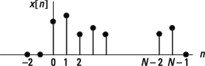
Figure 12-1: The finite duration signal x[n] used for establishing the DFT from the DTFT.

The DTFT of is the periodic function .

Consider at discrete frequencies :

where . The sampling of to produce is shown graphically in Figure 12-2a.

The use of WN here is an abbreviation for . In Chapter 11, represents the Fourier transform of a window function w[n]. Don’t let this dual use confuse you. WN is the standard notation for the complex weights, or twiddle factors, found in the DFT and FFT.

Figure 12-2: The DFT as sampling the DTFT (a) and sampling the z-transform (b).

From a z-transform perspective (see Chapter 14), the DFT also corresponds to sampling , the z-transform x[n], at uniformly spaced sample locations on the unit circle as shown in Figure 12-2b. Setting in X(z) reveals the DTFT, and sampling the DTFT at gives the DFT.

The DFT/IDFT Pair

The DFT is composed of a forward transform and an inverse transform, just like the Fourier transform (see Chapter 9) and the discrete-time Fourier transform (see Chapter 11). The forward transform is also known as analysis, because it takes in a discrete-time signal and performs spectral analysis. Here is the mathematical definition for the forward transform:

The complex weights are known as the twiddle factors. And the inverse discrete Fourier transform (IDFT) is sometimes called synthesis, because it synthesizes x[n] from the spectrum values, and is given by

The analysis and synthesis are often referred to as the DFT/IDFT pair. The transform is computable in both directions. This means that each sum is composed of just N terms. The number of complex multiplications and additions to compute all N points is thus finite, allowing for computer implementation. The same can’t be said about the continuous-time and discrete-time Fourier transform pairs, though, because they both involve integration over a continuous variable. This makes the DFT/IDFT very special.

Does the IDFT really undo the action of the DFT in exact mathematical terms? The best way to find out is to see for yourself.

Begin the proof by writing the definition of the IDFT and inserting the DFT in place of . Interchange sum orders and simplify:

To complete the proof, investigate the term in square brackets. You can use the finite geometric series (described in Chapter 2) to characterize this term

because for and for m = n, .

Throughout this chapter, I use the shorthand notation to indicate the relationship between and .

In the synthesis of from the ’s, you’re actually representing in terms of a Fourier series — or, more specifically, a discrete Fourier series (DFS) — with coefficients . The DFS point of view parallels the Fourier series analysis and synthesis pair of Chapter 8; only now you’re working in the discrete-time domain. Still, when one period of a signal is represented (or synthesized) by using its Fourier series coefficients, all the periods of the waveform are nicely sitting side by side along the time axis.

In the case of the DFT, you start with a finite length signal. But in the eyes of the DFT, all the adjoining periods are also present, at least mathematically. The signal periods on each side of the original N-point sequence are called the periodic extensions of the signal. Here’s the notation for the composite signal (a sequence of period N):

A compact notation for is . If you’re not familiar with the mod operator, think about any experience you may have with programming languages or digital electronics. The modN operator wraps the n value onto the interval by adding or subtracting integer multiples of N as needed. For example, 4 mod 10 = 4, 13 mod 10 = 3, and –5 mod 10 = 5.

On the frequency domain side, is also periodic, because the DTFT itself has period (see Chapter 11). With N samples of per period, the period of is also N. Formally, to maintain a duality relationship in the DFT/IDFT pair, you can also write this equation:

Example 12-1: To find the DFT of the four-point sequence , first assume, unless told otherwise, that a sequence being entered into the DFT starts at 0 and ends at . Here, . Working from the definition of the DFT, insert the sequence values in the sum formula:

Next, plug in to find , , , and .

Using Python and PyLab, you can access FFT functions via the fft package (no need to use import in the IPython environment). I use fft.fft(x,N) and fft.ifft(X,N) throughout this chapter to check hand calculations. For this example, a Python check reveals the following:

In [272]: fft.fft([2,2,1,1],4)

Out [272]: array([6.+0.j, 1.-1.j, 0.+0.j, 1.+1.j])# agree!

Example 12-2: Consider the DFT of the following pulse sequence, where :

In Chapter 11, the DTFT of is shown to be

Check out the continuous function magnitude spectrum for in Figure 12-3.

Figure 12-3: Magnitude spectrum plot of the DTFT for an pulse.

The DFT of is evaluated at , so

For the case of , shown in Figure 12-4, the results are somewhat unexpected because the most obvious shape resemblance to Figure 12-3 are the zero samples, which are correctly placed. There are no samples at the spectral peaks except at k = 0 and its periodic extensions.

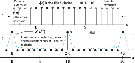
Figure 12-4: The sequence (a) and DFT (b) points for a pulse sequence with .

Figure 12-4 shows that sampling the DTFT with too few points results in a loss of spectral detail. The situation here is extreme. You’d hope that the DFT points would in some way represent the shape of the DTFT spectrum of Figure 12-3. Instead, spectral content is only at zero frequency (and multiples). The frequency domain samples at locations other than zero frequency hit the DTFT where it happens to null to zero.

Also notice that the with its periodic extensions (making it ) looks like a constant sequence. The input to the DFT is ten ones, so this sequence has absolutely no time variation. A constant sequence has all its spectral content located at zero frequency.

For the DFT to see some action, I pad the sequence with zeros, which makes the sequence I feed into the DFT look more like a pulse signal. Try and see what happens. Figure 12-5 has the same layout as Figure 12-4 but with .

Figure 12-5: The sequence (a) and DFT (b) points for a pulse sequence with and .

With twice as many samples, the DFT spectrum now has nonzero samples. The zero padding of the original x[n] allows the DFT to more closely approximate the true DTFT of x[n]. The underlying DTFT hasn’t changed because the nonzero points for the DFT are the same in both cases.

Figure 12-6 shows what happens when .

Here is PyLab code for generating the plot. Use the function signal.freqz() from the SciPy's signal package to approximate the DTFT of the sequence x. Inside freqz, you find the FFT is at work but with zero padding to 1,000 points.

In [288]: x = ones(10)

In [289]: w,X_DTFT = signal.freqz(x,1,arange(0,2*pi,pi/500))

In [290]: k_DFT = arange(0,80)

In [291]: X_DFT = fft.fft(x,80)

In [293]: plot(w,abs(X_DTFT))

In [296]: stem(k_DFT*2*pi/80,abs(X_DFT),'r','ro')

Figure 12-6: The DFT magnitude spectrum for and .

DFT Theorems and Properties

The discrete Fourier transform (DFT) has theorems and properties that are similar to those of the DTFT (Chapter 11) and z-transform (Chapter 14). A major difference of the DFT is the implicit periodicity in both the time and frequency domains. The theorems and properties of this section are summarized in Figure 12-7 with the addition of a few more useful DFT theorems.

Figure 12-7: DFT theorems and properties.

The first pair of properties that I describe in this section, linearity and symmetry, are parallel those of the DTFT, except in discrete or sampled frequency-domain form.

Two theorems that are distinctly different in behavior from their DTFT counterparts are circular sequence shift and circular convolution. The word circular appears in the theorem names, by the way, because of the periodic extension that’s present in the time domain when dealing with the IDFT. Circular sequence shift is the DFT version of the time delay theorem that I describe in Chapter 11, and circular convolution is the DFT version of the DTFT convolution theorem, also in Chapter 11.

The circular convolution theorem is powerful because it opens the door to the world of transform domain signal processing. In other words, the computational properties of the DFT/IDFT make it possible to implement a signal filtering system in the frequency domain by multiplying the signal spectrum samples times the filter frequency response and then calculating the inverse DFT to return to the time domain. (Find out how this works in the real world in the section “Application Example: Transform Domain Filtering,” later in this chapter.)

Carrying on from the DTFT

Linearity and frequency domain symmetry for real signals are two properties of the DFT that closely resemble their DTFT counterparts. The only differences are the discrete nature of the frequency domain and the fact that the time-domain signal has fixed length N.

The linearity theorem, , holds for the DFT — just as it does for all other transforms described in this book. But for linearity to make sense, all the sequence lengths must be the same.

For x[n] a real sequence, symmetry in the DFT domain holds as follows:

This equation represents conjugate symmetry, but with a circular index twist. The last line is the most useful in typical problem solving because it relates to the fundamental transform domain period, which lies on the interval . When you compute the N-point DFT of x[n] by using a computer tool, such as Python, the output is X[k] on the fundamental interval. Example 12-1 reveals that , so you may expect . True!

In terms of magnitude and phase:

For real sequences, the DFT is unique over just the first points, which parallels the DTFT for real signals being unique for (see Chapter 11). You can verify this directly from .

Consider the following listing of the X[k] points, where I use to relate point indexes above N/2 to those less than or equal to N/2. The case of N even means the point at N/2 is equal to itself (N – N/2 = N/2), and for N odd, the point N/2 doesn’t exist.

Circular sequence shift

The time shift theorem for the DTFT says (see Chapter 11). For the DFT, things are different due to the characteristics of the DFT. It can be shown that .

Example 12-3: Sketch for an arbitrary eight-point sequence. See Figure 12-8 for a series of four waveform plots, starting with and ending with .

PyLab's roll(x,m) function makes checking the numbers easy:

In [313]: x

Out[313]: array([0, 1, 2, 3, 4, 5, 6, 7])

In [314]: roll(x,3) # -3 rolls left by 3

Out[314]: array([5, 6, 7, 0, 1, 2, 3, 4])

Figure 12-8: Circular shift by three of an eight-point sequence: (a), (b), (c), and (d).

---

---

Circular convolution

Suppose that N-point sequences and have DFTs and , respectively. Consider the product . You may guess that , the inverse DFT of , is the convolution of with because convolution in the time domain is multiplication in the frequency domain (covered in Chapters 9 and 10). But it turns out that this assumption is only partially correct.

Because the IDFT of X1[k] and X2[k] produces periodic extensions of and , the convolution sum, first developed in Chapter 6, is replaced by a circular, or periodic, convolution. The word circular is used because the periodic extensions show that time-domain signal values are imprinted on a cylinder (cross-section is a circle); as that cylinder rolls along the time axis, it imprints the same signal over and over again.

It can be shown that x3[n] is a circular convolution sum having mathematical form:

Notice the use of the periodic extension signals in the argument of the sum and the fact that the sum limits run over just the fundamental interval . The signal x3[n] can also be viewed with periodic extensions.

---

---

A short-hand notation for circular convolution is .

Doing the actual circular convolution isn’t the objective. The DFT/IDFT is a numerical algorithm in both directions. Do you see integrals anywhere? You can implement the convolution in the frequency domain as a multiplication of transforms (DFT-based frequency domain) and then return to the time domain via the IDFT. Figure 12-9 shows a block diagram that describes circular convolution in the frequency domain.

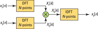
Figure 12-9: N-point circular convolution as multiplication in the frequency (DFT) domain.

Practicing with short length circular convolutions is instructive, and it makes it easier to appreciate the utility of DFT/IDFT.

Example 12-4: Consider the four-point circular convolution of the sequences and , shown in Figure 12-10.

Figure 12-10: Two four-point sequences used for circular convolution.

Find the output by hand, calculating with the help of the waveform sketches in Figure 12-11. The filled stems represent the sequence values that need to be pointwise multiplied over the interval . For , the sum of products is .

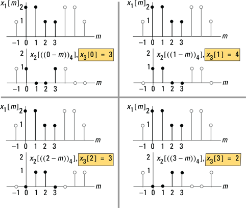
Figure 12-11: The hand calculation of a four-point circular convolution.

Now you can work the circular convolution in the DFT domain, using Pylab as the numerical engine for the DFT and IDFT:

In [316]: x1 = [2,2,1,1]

In [317]: x2 = [1,1,0,0]

In [318]: X3 = fft.fft(x1)*fft.fft(x2)

In [319]: X3

Out[319]: array([12.+0.j, 0.-2.j, 0.+0.j, 0.+2.j])

In [320]: x3 = fft.ifft(X3)

In [321]: x3

Out[321]: array([3.+0.j, 4.+0.j, 3.+0.j, 2.+0.j])

The Python results agree with the hand calculation.

A more rigorous check is to actually perform the DFT and IDFT calculations by hand. The four-point transforms aren’t too difficult. The sequence in Example 12-1 is , so you have . Next, you find X2[k] and then multiply the DFTs point by point. In the final step, you apply the IDFT to the four-point sequence to get x3[n].

Computing the DFT with the Fast Fourier Transform

The fast Fourier transform (FFT) is one of the pillars of modern signal processing because the DFT via an FFT algorithm is so efficient. You’ll find it hard at work during the design, simulation, and implementation phase of all types of products.

For example, the FFT makes quick work of calculating the frequency response and input and output spectra of signals and systems. The functions available in Python’s PyLab, as well as other popular commercial tools, routinely rely on this capability. And at the implementation phase of a design, you may use the FFT to perform transform domain filtering, get real-time spectral analysis, or lock to a GPS signal to get a position fix. The test equipment you use on the lab bench to verify the final design may use the FFT, and modern oscilloscopes use the FFT to display the spectrum of the waveform input to the instrument. The application list goes on and on, and the common thread is efficient computation by using computer hardware.

In this section, I point out the benefits of the FFT by looking at the computation burden that exists without it. I also describe the decimation-in-time (DIT) FFT algorithm to emphasize the computational performance gains that you can achieve with FFT algorithms. The DFT, or forward transform, is the focus here, but a modified version of the FFT algorithm can easily calculate the IDFT, too!

From the definition of the DFT, the number of complex multiplies and adds required for an N-point transform is and , respectively. The goal of the FFT is to significantly reduce these numbers, especially multiplication count.

Decimation-in-time FFT algorithm

Of the many FFT algorithms, the basic formula is the radix-2 decimation-in-time (DIT) algorithm, in which N must be a power of 2. If you let , where v is a positive integer, then N = 8 and v = 3. A property of the radix-2 FFT is that you can break down the DFT computation into stages of two-point DFTs per stage. The fundamental computational unit of the radix-2 FFT is a two-point DFT.

Figure 12-12a is a signal flowgraph (SFG) of an eight-point FFT that illustrates the complete algorithm. The SFG, a network of directed branches, is a way to graphically depict the flow of input signal values being transformed to output values. For the case of the FFT, the SFG shows you that N signal values x[0] through x[N – 1] enter from the left and exit at the far right as the transformed values X[1] through X[N – 1].

Signal branches contain arrows to denote the direction of signal flow. When a signal traverses a branch, it’s multiplied by the twiddle factor (a term referencing a complex constant) that’s next to the branch arrow in Figure 12-12. The absence of a constant next to an arrow means that you need to multiply the signal by one.

The nodes of the SFG are the open circles where branches enter and depart. When more than one branch enters a node, the signal value at that node is the sum of branch values entering the node. For the case of the FFT SFG, the nodes also delineate the stages of the FFT. A node with no entering branches is called a source node (the input signal injection point), and a node with only entering branches is called a sink node (the output signal extraction point).

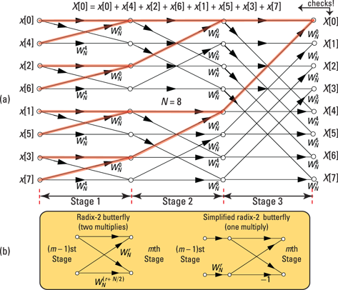
Figure 12-12: An eight-point radix-2 FFT signal flowgraph (a) and a simplified radix-2 ­butterfly (b).

At each stage of the SFG are four radix-2 butterflies, similar to the two-­multiplier version of Figure 12-12b (they’re especially visible at Stage 1). The radix-2 butterfly is actually a two-point DFT; the radix-2 FFT is composed of two-point DFTs.

To demonstrate that the FFT is correct for the N = 8 case, consider X[0]. From the definition of the DFT

In the SFG of Figure 12-12, I shaded the branches from each input x[n] to the output X[0]. The branch gain applied to each input is unity. Branch values entering a node sum X[0] is the sum of all the x[n] values entering the SFG, so this agrees with the direct DFT calculation given earlier in this section.

Feel free to check the paths leading to any other output node and see that the DFT definition of the section “Establishing the Discrete Fourier Transform” is satisfied.

Referring again to Figure 12-12b, the radix-2 butterfly on the left may be replaced by a simplified butterfly that requires only one complex multiply. When using the simplified radix-2 butterfly, each stage requires complex multiplies. If there are log2N stages, then the total complex multiply count is . Find a comparison of DFT and FFT multiply complexity in Figure 12-13.

Figure 12-13: DFT versus radix-2 FFT complex multiplication count.

The speed-up factor of the FFT as N increases is impressive, I think. As a bonus, all computations of the FFT of Figure 12-12 are in-place. Two values enter each butterfly and are replaced by two new numbers; there’s no need to create a working copy of the N-input signal values, hence the term in-place computation.

Working variables can be kept to a minimum. The in-place property comes at the expense of the input signal samples being scrambled. This scrambling is actually just a bit of reversing of the input index. For example:

Computing the inverse FFT

If you’re wondering about efficient computation of the IDFT, rest assured that it’s quite doable. To find the inverse FFT (IFFT), you follow these steps:

1. Conjugate the twiddle factors.

Because the FFT implements the DFT, you can look at this mathematically by making the twiddle factor substitution in the definition of the DFT as a check:

2. Scale the final output by N.

Make this substitution in the already modified DFT expression: . On the right side is the definition of the IDFT (provided in the earlier section “The DFT/IDFT Pair” with x[n] in place of X[n]).

The software tools fully support this, too. In the Python portion of Example 12-4, I use the function called fft.fft(x,N) for the FFT (and hence DFT) and fft.ifft(X,N) for the IFFT (the IDFT).

Application Example: Transform Domain Filtering

Filtering a signal with finite impulse response entirely in the frequency domain is possible by using the DFT/IDFT. Here are two questions you must answer to complete this process:

How do I make circular convolution perform ordinary linear convolution, or the convolution sum (introduced in Chapter 6)?

How do I handle a very long sequence while keeping the DFT length manageable?

In this section, I point out how circular convolution can be made to act like linear convolution and take advantage of the computation efficiency offered by the FFT. I also tell you how to use the FFT/IFFT to continuously filter a discrete-time signal, using a technique known as overlap and add, which makes it possible to filter signals in the frequency domain. This isn’t simply an analysis technique; it’s a real implementation approach.

Making circular convolution perform linear convolution

The linear convolution of a length L signal with a length P sequence results in a signal of length (see Chapter 6). With circular convolution, both signal sequences need to have length N, and the circular convolution results in a length N sequence.

Can circular convolution emulate linear convolution? The answer is yes if you zero pad x[n] and h[n] to length .

Zero padding means you append zero signal values to the end of a signal: {x[0], x[1], . . . , so x[L – 1]} becomes {x[0], x[1], . . . , x[L – 1], 0, 0, . . . , 0}, and the number of appended zero values is N – L. For the length P sequence h[n], you zero pad by appending N – P zero values.

Zero padding is a big deal because it allows you to use circular convolution to produce the same result as linear convolution. In practice, circular convolution happens in the frequency domain, using the block diagram of Figure 12-8.

Using overlap and add to continuously filter sequences

Assume that is a sequence of possibly infinite duration and is a length P FIR filter. Divide into segments of finite length L and then filter each segment by using the DFT/IDFT.

You can complete the segment filtering by using zero padded length transforms. Afterward, add the filtered sections together — with overlap because . This process requires the following steps:

1. Decompose , as shown in Figure 12-14.

2. Compute the DFT (actually use an FFT) of each subsequence in Figure 12-15 as they’re formed with increasing n.

Also compute , or you may specify H[k] directly in the frequency domain.

3. Multiply the frequency domain points together: Xr[k]H[k] for each r.

4. Take the IDFT of the overlapping frequency domain subsequences Xr[k]H[k] to produce , and then overlap and add the time domain signal sequences as shown in Figure 12-15.

The function y = OA_filter(x,h,N) in the module ssd.py implements overlap and add (OA). A variation on OA is overlap and save (OS), which you can also find in ssd.py as OS_filter(x,h,N).

Figure 12-14: Segmenting with zero padding to avoid time aliasing in the transform-domain convolution.

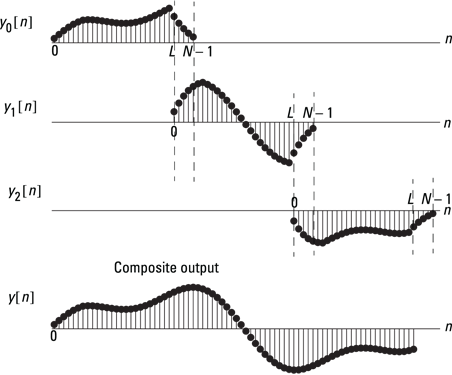
Figure 12-15: The final step in the overlap-add method is to overlap and add the yr[n] subsequences.