Chapter 13

The Laplace Transform for Continuous-Time

In This Chapter

Checking out the two-sided and one-sided Laplace transforms

Getting to know the Laplace transform properties

Inversing the Laplace transform

Understanding the system function

The Laplace transform (LT) is a generalization of the Fourier transform (FT) and has a lot of nice features. For starters, the LT exists for a wider class of signals than FT. But the LT really shines when it’s used to solve linear constant coefficient (LCC) differential equations (see Chapter 7) because it enables you to get the total solution (forced and transient) for LCC differential equations and manage nonzero initial conditions automatically with algebraic manipulation alone.

Unlike the frequency domain, which has real frequency variable f or , the LT transforms signals and linear time-invariant (LTI) impulse responses into the s-domain, where s is a complex variable. This means you can avoid using the convolution integral by simply multiplying the transformed quantities in the s-domain. The impulse response of an LCC differential equation is a ratio of polynomials in s (rational function). The denominator roots are the poles, and the numerator roots are the zeros. And a system’s poles and zeros reveal a lot about the system, including whether it’s stable and what the frequency response’s shape is.

Returning from the s-domain requires an inverse LT procedure. In this chapter, I describe the two forms of the Laplace transform. I also tell you how to apply the Laplace transform by using partial fraction expansion and table lookup. Check out Chapter 2 for a math refresher if you think you need it.

Seeing Double: The Two-Sided Laplace Transform

Signals and systems use two forms of the Laplace transform (LT): the two-sided and the more specific one-sided. In this section, I introduce the basics of the two-sided form before diving into its one-sided counterpart.

The two-sided LT accepts two-sided signals, or signals whose extent is infinite for both t < 0 and t > 0. This form of the LT is closely related to the FT, which also accepts signals over the same time axis interval. But the two-sided LT can work with both causal and non-causal system models; the one-sided LT can’t. The drawback of the two-sided form is that it’s unable to deal with systems having nonzero initial conditions.

The two-sided LT takes the continuous-time signal x(t) and turns it into the s-domain function:

where is a complex variable and the subscript in denotes the two-sided LT.

It’s no accident that I chose as the real axis variable and as the imaginary axis variable. The use of for the real axis name is almost universal in the signals and systems community. The imaginary axis is because of the connection to the FT.

You can find the relationship to the radian frequency FT by writing

The two-sided LT is always equivalent to the FT of signal x(t) multiplied by an exponential weighting factor . This factor allows improved convergence of the LT. If, however, the FT of exists, it’s a simple matter to set in the equation and see that . This relationship is shown in Figure 13-1.

Finding direction with the ROC

The LT doesn’t usually converge over the entire s-plane. The region in the s-plane for which the LT converges is known as the region of convergence (ROC). Uniform convergence requires that

Figure 13-1: The -axis in the s-plane and the relation between and .

Convergence depends only on , so if the LT converges for , then the ROC also contains the vertical line . It can be shown that the general ROC for a two-sided signal is the vertical strip in the s-plane, as shown in Figure 13-2.

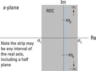
Figure 13-2: The general ROC is a vertical strip controlled by .

You can determine the value of and by the nature of the signal or impulse response being transformed. That both and/or is also possible.

To show that the ROC is a vertical strip in the s-plane for x(t) two-sided, first consider x(t) is right-sided, meaning x(t) = 0 for t < t1. If the LT of x(t) includes the vertical line , it must be that . The ROC must also include because the integral is finite. What makes this true is the fact that for t > 0 and t1 finite. You can generalize this result for to say for x(t) right-sided, the ROC is the half-plane .

If x(t) is left-sided, meaning x(t) = 0 for t > t2 and the LT of x(t) includes the vertical line , you can show, through an argument similar to the right-sided case, that the ROC is the half-plane .

Finally, for x(t) two-sided, the ROC is the intersection of right and left half-planes, which is the vertical strip , provided that ; otherwise, the ROC is empty, meaning the LT isn’t absolutely convergent anywhere.

Example 13-1: Find the two-sided LT of the right-sided signal , where a may be real or complex. Note that right-sided means the signal is 0 for . A further specialization of right-sided is to say that a signal is causal, meaning . Use the definition of the two-sided LT:

Example 13-2: Find the two-sided LT of the left-sided signal , where a may be real or complex. Left-sided means the signal is 0 for . Another way to refer to a left-sided signal is to say it’s anticausal, meaning (the opposite of causal). Note that a non-causal signal is two-sided. Use this definition to reveal ROC: Re{s} < –Re{a}.

Both of Example 13-1 and of Example 13-2 have the same LT! The ROCs, however, are distinct — they’re complementary regions — making the LTs distinguishable only by the ROCs being different. The purpose of Example 13-2 is to point out that, without the ROC, you can’t return to the time domain without ambiguity — is the signal left-sided or right-sided?

Locating poles and zeros

When the LT is a rational function, as in Examples 13-1 and 13-2, it takes the form , where and are each polynomials in s. The roots of — where — are the zeros of , and the roots of are the poles of .

Think of the poles and zeros as the magnitude of a 3D stretchy surface placed over the s-plane. The surface height ranges from zero to infinity. At the zero locations, because N(s) = 0, the surface is literally tacked down to zero. At the pole locations, because D(s) = 0, you have , which you can view as a tent pole pushing the stretchy surface up to infinity. It’s not your average circus tent or camping tent, but when I plot the poles and zeros in the s-plane, I use the symbols and O.

Take a look at the pole-zero plots of and , including the ROC, in Figure 13-3.

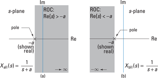
Figure 13-3: The pole-zero plot and ROC of (a) and (b) of Examples 13-1 and 13-2, respectively.

Checking stability for LTI systems with the ROC

An LTI system is bounded-input bounded-output (BIBO) stable (see Chapter 5) if .

Transforming to the s-domain has its perks. Here’s what I mean: The LT of the impulse response is called the system function. The Fourier transform of the impulse response is the frequency response (covered in Chapter 9), and the system function generalizes this result to the entire s-plane. The frequency domain is just the Laplace domain evaluated along the axis. It can be shown that if the ROC of contains the -axis, then the system is BIBO stable. Cool, right?

The proof follows by expanding , using the triangle inequality — a general mathematical result that states that the magnitude of the sum of two quantities is less than or equal to the sum of the magnitudes:

The triangle inequality reveals that the magnitude of a sum is bounded by the sum of the magnitudes.

Checking stability of causal systems through pole positions

The poles of must sit outside the ROC because the poles of are singularities. In other words, is unbounded at the poles. For right-sided (and causal) systems, the ROC is the region to the right of the vertical line passing through the pole with the largest real part. In Example 13-1, this represents all the values greater than .

An LTI system with impulse response and system function is BIBO stable if the ROC contains the -axis. For the special case of a causal system, when for , the poles of must lie in the left half of the s-plane, indicating a negative real part, because causal sequences have ROC positioned to the right of a line passing through the pole with the largest real part. In short, a causal LTI system is stable if the poles lie in the left-half plane (LHP).

Digging into the One-Sided Laplace Transform

The one-sided Laplace transform (LT) offers the capability to analyze causal systems with nonzero initial conditions and inputs applied, starting at . Unlike two-sided LT signals, the one-sided LT doesn’t allow you to analyze signals that are nonzero for . The trade-off is acceptable because the transient analysis of causal LTI systems in the s-domain involves only algebraic manipulations.

The one-sided LT restricts the integration interval to :

Use the to accommodate signals such as the impulse and the step (see Chapter 5). To be clear, is as approaches zero.

All the results developed for the two-sided LT in the previous section hold under the one-sided case as long as the signals and systems are causal — that is, both and are zero for . The poles of must lie in the left-half plane for stability.

Example 13-3: To find the LT of , use the definition and the sifting property of the following impulse function:

The ROC is . In terms of , the ROC is just . This means that the ROC includes the entire s-plane. And when , the is needed to properly handle the integral of .

Example 13-4: Find the LT of . This signal is causal, so the one-sided and two-sided LTs are equal because the step function, , makes the integration limits identical.

Use Example 13-1 and set :

The ROC doesn’t include the -axis because a pole is at zero.

Example 13-5: To find the system function corresponding to the impulse response , first recognize that linearity holds for the LT: .

Again, use Example 13-1, where two-sided and one-sided signals are identical:

One zero and two poles exist in this solution: . You can find the ROC for the solution as a whole by intersecting the ROC for each exponential term. Just use the ROC from Example 13-1:

The pole with the largest real part sets the ROC boundary. The system is stable because the ROC includes the -axis. But a more memorable finding is the fact that the poles are in the left-half s-plane, which indicates that this causal system is stable.

Checking Out LT Properties

Problem solving with the LT centers on the use of transform theorems and a reasonable catalog of transform pairs. Knowing key theorems and pairs can help you move quickly through problems, especially when you need an inverse transform. In this section, I point out some of the most common LT theorems and transform pairs.

The theorems and transform pairs developed in this section are valid for the one-sided LT. Those applicable to the two-sided LT are different in some cases.

Transform theorems

In this section of basic theorems, assume that the signals and systems of interest are causal.

Find a collection of significant one-sided Laplace transform theorems in Figure 13-4.

Figure 13-4: One-sided Laplace transform theorems.

Delay

The one-sided LT of a signal with time delay t0 > 0 is an important modeling capability. To set up the theorem, consider for :

Example 13-6: Suppose that is a periodic-like waveform with period . A true periodic waveform has periods extending to as well. Here, the signal is causal with the first period starting at :

To find , write .

Taking the LT of both sides results in the following equation:

Differentiation

The differentiation theorem is fundamental in the solution of LCC differential equations with nonzero initial conditions. If you start with , you ultimately get a result for . Using integration by parts, you can show that

---

---

Using mathematical induction, you can then show the following, where :

Integration

The integration theorem is the complement to the differentiation theorem. It can be shown that

Example 13-7: Find the LT of the ramp signal . The study of singularity functions (see Chapter 3) reveals that the step function u(t) is the integral of the impulse function. If you integrate the step function, you get the ramp function. In the s-domain, the LT of a step function is 1/s, so applying the integration theorem shows that

This is a repeated pole at s = 0 with the ROC the right-half plane.

Convolution

Given causal , the convolution theorem states that . This theorem is fundamental to signals and systems modeling, because it allows you to study the action of passing a signal through a system in the s-domain. An even bigger deal is that convolution in the time domain is multiplication in the s-domain. The FT convolution theorem (see Chapter 9) provides this capability, too, but the LT version is superior, especially when your goal is to find a time-domain solution.

s-shift

Solving LCC differential equations frequently involves signals with an exponential decay. The s-shift theorem provides this information:

The s-shift moves all the poles and zeros of to the left by . The left edge of the ROC also shifts to the left by . Stability improves!

---

---

Example 13-8: To find with implied as a result of the one-sided LT, start with . Using linearity, Euler’s inverse formulas for sine and cosine, and the transform pair developed in Example 13-1, solve for the LT:

Finally, let :

The poles that were at shift to . The ROC for both transforms is .

---

---

Final value

The final value theorem states that if the limit exists — or x(t) reaches a bounded value only if the poles of lie in the left-half plane (LHP). This theorem is particularly useful for determining steady-state error in control systems (covered in Chapter 18). You don’t need a complete inverse LT just to get .

Example 13-9: Apply the final value theorem to :

What’s wrong with the analysis of ? Poles on the -axis () make oscillate forever. The limit doesn’t exist because the poles of don’t lie in the LHP, so the theorem can’t be applied. The moral of this story is to study the problem to be sure the theorem applies!

Transform pairs

Transform pairs play a starring role in LT action. After you see the transform for a few signal types, you can use that result the next time you encounter it in a problem. This approach holds for both forward and inverse transforms (see the section “Getting Back to the Time Domain,” later in this chapter). Figure 13-5 highlights some LT pairs.

Figure 13-5: Laplace transform pairs.

Example 13-10: Develop a transform pair where the time-domain signal is a linear combination of exponentially damped cosine and sine terms. You need this pair when finding the inverse Laplace transform (ILT) of a rational function X(s) containing a complex conjugate pole pair (see Example 13-12 for a full example).

The starting point from the s-domain side is , with to ensure complex conjugate poles. You can write the time-domain solution as a linear combination of the time-domain side of transform pairs in Lines 7 and 8 of Figure 13-5: . Your objective is to find a and b in terms of the coefficients of X(s). You can do so with the following steps:

1. Equate X(s) with a linear combination of the s-domain side of transform pairs in Lines 7 and 8 of Figure 13-5 by first matching up the denominators in

Recall the old algebra trick called completing the square, in which, given a quadratic polynomial , you rewrite it as , where c1 and c2 are constants. You then equate like terms:

So and or .

2. Find a and b by matching like terms in the numerator: and or .

As a test case, consider . Using the equations for , a, and b in Steps 1 and 2, you find that , a = 1, and ; for example:

On the time-domain side, you have

To check this with Maxima you use the ILT function ilt() and find agreement when using the original X(s) function:

Getting Back to the Time Domain

Working in the s-domain is more of a means to an end than an end itself. In particular, you may bring signals to the s-domain by using the LT and then performing some operations and/or getting an s-domain function; but in the end, you need to work with the corresponding time-domain signal.

Returning to the time domain requires the inverse Laplace transform (ILT). Formally, the ILT requires contour integration, which is a line integral over a closed path in the s-plane. This approach relies on a complex variable theory background.

In this section, I describe how to achieve contour integration by using partial fraction expansion (PFE) and table lookup. I also point out a few PFE considerations and include examples that describe how these considerations play out in the real world.

The general formula you need to complete the ILT is

The first step is to ensure that is proper rational, that . If it isn’t, you need to use long division to reduce the order of the denominator. After long division, you end up with this:

is the remainder, having polynomial degree less than N.

Dealing with distinct poles

If the poles are simple (unrepeated) and is proper rational, you can write , where the represents the nonzero poles of . Find the PFE coefficients by using the residue formula: (see Chapter 2).

If you need to perform long division (such as when the order of the numerator polynomial is greater than or equal to the order of the denominator polynomial), be sure to augment your final solution with the long division terms .

Working double time with twin poles

When has the pole repeated once (a multiplicity of two), the expansion form is augmented as follows:

You can find the coefficients by using the residue formula. The formula for

is and is found last by substitution. See Example 13-11.

Completing inversion

For the general ILT scenario outlined at the start of the section, invert three transform types via table lookup. The first manages the long division result; the second, distinct poles; and the third, poles of multiplicity two:

Using tables to complete the inverse Laplace transform

This section contains two ILT examples that describe how to complete PFE with the table-lookup approach. The first example, Example 13-11, considers a repeated real pole; the second, Example 13-12, considers a complex conjugate pole pair. Both examples follow this step-by-step process:

1. Find out whether X(s) is a proper rational function; if not, perform long division to make it so.

2. Find the roots of the denominator polynomial and make note of any repeated poles (roots) and/or complex conjugate poles (roots).

3. Write the general PFE of X(s) in terms of undetermined coefficients.

For the case of complex conjugate pole pairs, use the special transform pair developed in Example 13-9 so the resulting time domain is conveniently expressed in terms of exponentially damped cosine and sine functions.

4. Solve for the coefficients by using a combination of the residue formula and substitution techniques as needed.

5. Apply the ILT to the individual PFE terms, using table lookup.

6. Check your solution by using a computer tool, such as Maxima or Python.

Example 13-11: Find the impulse response corresponding to a system function containing three poles: one at s = –2 and two at s = –1, and one zero at s = 0. Specifically, H(s) is the proper rational function .

1. Use the repeated roots form for PFE to expand H(s) into three terms:

2. Find the coefficients R1 and S2, using the residue formula as described in section “Working double time with twin poles”:

3. Solve for by direct substitution. Let :

4. Place the values you found for R1, S1, and S2 into the expanded form for H(s) of Step 1, and then apply the ILT term by term:

Check the results with Maxima to see that all is well:

Example 13-12: Find the impulse response corresponding to a system function that has one real pole and one complex conjugate pair. Here’s the equation for a third-order system function with pole at s = –1 and complex conjugate poles at :

All the poles are distinct, so you can use the residue formula to find the PFE coefficients and the impulse response. This approach results in real and complex exponential time-domain terms — not a clean solution without further algebraic manipulation. But the impulse response is real because all the poles are either real or complex conjugate pairs, so the complex exponentials do reduce to real sine and cosine terms.

For this scenario, I recommend using the s-shift theorem and the associated transform pairs found in the earlier section “s-shift,” because this approach takes you to a usable time-domain solution involving damped sine and cosine terms. Example 13-10 boiled all of this down to a nice set of coefficient equations. The PFE expansion for the conjugate pole term is . You can find the equations for , a, and b in Example 13-10.

Now it’s time for action. Here’s the process:

1. For the three-pole system, complete the square of the complex conjugate pole term.

Use the equations from Step 1 of Example 13-10, noting that, here, a1 = 2 and a0 = 2: and . Write the PFE as

2. Solve for by using the residue formula; then use variable substitution to find a and b.

3. Solve the two equations for the unknowns to find .

Use the transform pairs Lines 3, 7, and 8 in Figure 13-5 to get the inverse transform of the three terms:

Checking with Maxima shows agreement:

Working with the System Function

The general LCC differential equation (see Chapter 7) is defined as

By taking the LT of both sides of this equation, using linearity and the differentiation theorem (described in the section “Transform theorems,” earlier in this chapter), you can find the system function as the ratio of .

This works because of the convolution theorem (see Figure 13-4), or .

Assuming zero initial conditions, you use the differentiation theorem (see Figure 13-4) to find the LT of each term on the left and right sides of the general LCC differential equation. You then factor out Y(s) and X(s) and form the ratio Y(s)/X(s) = H(s) on the left side, and what remains on the right side is the system function:

After you solve for , you can perform analysis of the system function alone or in combination with signals.

Plot the poles and zeros of H(s) and see whether the poles are in the left-half plane, making the system stable.

Assuming the system is stable, plot the frequency response magnitude and phase by letting in H(s) to characterize the system filtering properties.

Find the inverse LT to get the impulse response, — the core time-domain characterization of the system.

Find the inverse LT to get the step response.

Find the inverse LT to get the output in response to a specific input .

You can also work initial conditions into the solution by not assuming zero initial conditions in the earlier system function analysis.

Managing nonzero initial conditions

A feature of the one-sided LT is that you can handle nonzero initial conditions when solving the general LCC differential equation. The key to this is the differentiation theorem. The lead term snX(s) is the core result of the theorem, but the nonzero initial conditions are carried by the terms , k = 0, … , n – 1.

Example 13-13: The input to an LTI system is given by , and the system LCC differential equation is . To find the system output with nonzero initial conditions, follow these steps:

1. Apply the differentiation theorem (see Figure 13-4) to both sides of the LCC differential equation:

2. Solve for , making substitutions for and :

Use Line 3 of Figure 13-5: .

3. Solve for the partial fraction coefficients R1 and R2:

4. Insert the coefficients into the PFE for Y(s) and then apply the inverse Laplace transform to each term:

Check Maxima to see whether it agrees:

Checking the frequency response with pole-zero location

The location of the poles and zeros of a system controls the frequency response — . Consider the following:

pk and zk are the poles and zeros of H(s) and and are the frequency response contributions of each pole and zero. The vectors point from the zero and pole locations to on the imaginary axis. This provides a connection between the pole-zero geometry and the frequency response. In particular, the ratio of vector magnitudes, , is the magnitude response. The phase response is .

Example 13-14: Consider the simple first-order system:

The single numerator and denominator vectors indicates that the geometry is rather simple. You can use the software app PZ_Geom_S to further explore the relationship between frequency response and pole-zero location. Check out the screen shot of PZ_geom_S in Figure 13-6.

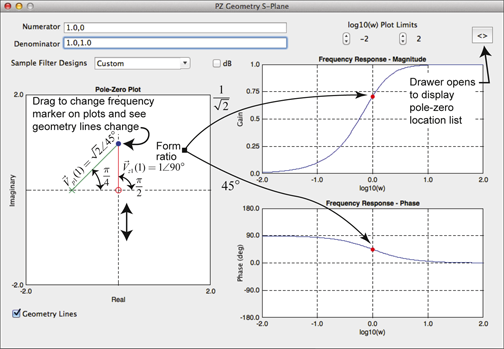
Figure 13-6: The app PZ-Geom_S displaying the pole-zero geometry for .