Chapter 15

Putting It All Together: Analysis and Modeling Across Domains

In This Chapter

Looking at the big picture of signals and systems domains

Working with LCCDEs across both continuous- and discrete-time domains

Tackling signals and systems problems beyond the one-liner solution

Working across domains is a fact of life as a computer and electronic engineer. Solving real computer and electrical engineering tasks requires you to assimilate the vast array of signals and systems concepts and techniques and apply them in a smart and efficient way. For many people, putting everything together and coming up with real solutions is tough. My goal in this chapter is to help you see how various concepts interact and function in actual situations.

When you receive design requirements for a new project, the system architecture will likely contain a variety of subsystems that cover both continuous- and discrete-time. A powerful subsystem building block is the linear constant coefficient (LCC) differential equation and the LCC difference equation. These subsystems are responsible for implementing what are commonly referred to as filters.

Filters allow some signals to pass and they block others. For design and analysis purposes, you can view filters in the time, frequency, and s- and z-domains (see Chapters 7, 9, 11, 13, and 14 for details on how filters function in the specific domains). Or system design constraints may result in a filter design that’s distributed between the continuous and discrete domains.

This chapter explores two common scenarios that require you to work across domains t, f, and s for continuous-time signals and systems and across n, , and z-domains for discrete time as well as function between continuous and discrete domains as a whole. I point out how to approach these situations and use analysis techniques that draw upon powerful software tool sets.

The systems-level problems in this chapter require you to have an approach in mind before moving forward with specific action steps. Yet arriving at a solution approach gets a bit hairy when real problems are complex. Eventually, experience can guide you to the best approaches.

In the meantime, here are some general problem-solving guidelines:

Create a system block diagram from the problem statement.

Create detailed subsystem models for critical areas in the design.

Start with simple behavioral level models for perceived non-critical subsystems.

Through analysis, get a first-cut design of the critical subsystem(s).

Verify composite system performance via a high-level analysis model and simulation.

Relating Domains

To successfully apply the various signals and systems concepts as part of practical engineering scenarios, you need to know what analysis tools are available. Figure 15-1 shows the mathematical relationships between time, frequency, and the s- and z-domains as described in Chapters 1 through 14 of this book. This portrayal offers perspective on a well-rounded study of signals and systems and reveals that you can establish relationships between domains in more than one way.

When working through engineering problems, I recommend staying on a single branch when possible — but sometimes you just can’t. Fortunately, if you need to go from the time domain t to the discrete-time frequency domain , you can hop from t to n and then from n to or go from t to f and then f to .

Some of the interconnects in Figure 15-1 are simply conceptual; they don’t hold mathematically under all conditions. For example, Fourier transforms in the limit (see Chapters 9 and 11 for continuous- and discrete-time signals) make it invalid to sample the s- or z-domains by letting and . Figure 15-1 tells you that the region of convergence (ROCs) must include the frequency axis for this connection to be valid. Sampling theory offers the links between t and n, but a causal interpolation filter leads to less than perfect reconstruction, revealing that the idea of exact is conceptual only. An approximation is used in real-world systems.

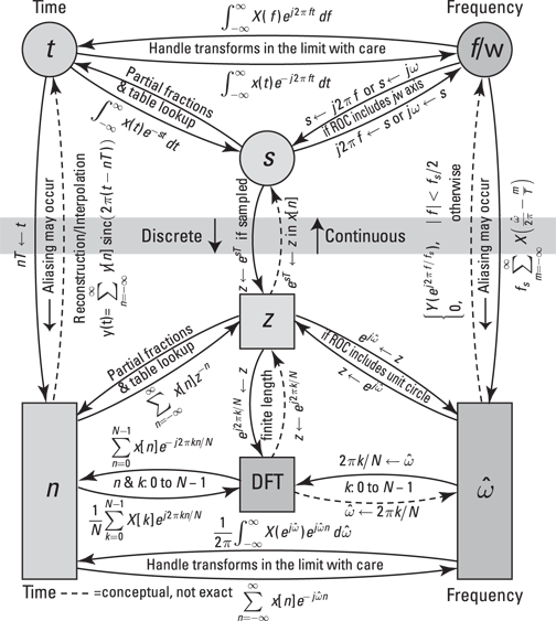
Figure 15-1: The signals and system math of working across both continuous and discrete domains.

Using PyLab for LCC Differential and Difference Equations

Computer tools play a big part in modern signals and systems analysis and design. LCC differential and difference equations (covered in Chapters 7, 9, 11, 13, and 14) are a fundamental part of simple and highly complex systems. Fortunately, current software tools make it possible to work across domains with these LCC equations without too much pain.

LCC differential and difference equations are completely characterized by the {ak} and {bk} coefficient sets (find details on coefficient sets in Chapter 7). You can use such tools as Pylab with the SciPy signal package to design high performance filters, particularly in the discrete-time domain. The filter design functions of signal give you the {ak} and {bk} coefficients in response to the design requirements you input. You can then use the filter designs in the simulation of larger systems.

Throughout this book, I use the open-source tool PyLab and its various pieces. In this section, I provide information on how to use the PyLab tools to design and analyze LCC differential and difference equations systems across the continuous- and discrete-time domains.

Continuous time

Three representations of the LCC differential equation system are the time, frequency, and s-domains, and the same coefficient sets, {bk} and {ak}, exist in all three representations. Here are the corresponding input and output relationships in these domains:

Time domain (from differential equation):

Time domain (from impulse response):

Frequency domain:

s-domain:

In the second line of the differential equation, the impulse response, h(t), along with the convolution integral of Chapter 5 produce the output, y(t), from the input, x(t). In the third line, the convolution theorem for Fourier transforms (Chapter 9) produces the output spectrum, Y(f), as the product of the input spectrum, X(f), and the frequency response, H(f) — which is the Fourier transform of the impulse response. In the fourth line, the convolution theorem for Laplace transforms (Chapter 13) produces the s-domain output, Y(s), as the product of the input, X(s), and the system function, H(s) — which is the Laplace transform of the impulse response.

Figure 15-2 highlights the key functions in PyLab and the ssd.py code module you can use to work across continuous-time domains. Remember, these functions are at the top level. You can integrate many lower-level functions (such as math, array manipulation, and plotting library functions) with these top-level functions to carry out specific analysis tasks.

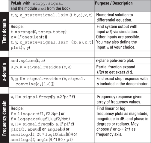
Figure 15-2: Working with LCC differential equations across domains using PyLab.

Here’s what you can find in Figure 15-2:

The time-domain rows show a recipe to solve the differential equation numerically by using signal.lsim((b,a),x,t) for a step function input. The arrays b and a correspond to the coefficient sets {bk} and {ak}. Input signals of your own choosing are possible, too. The time-domain simulation allows you to characterize a system's behavior at the actual waveform level.

In the s-domain rows, find the pole-zero plot of the system function H(s) by using ssd.splane(b,a). Also find out how to solve the partial fraction expansion (PFE) of H(s) and H(s)/s to get a mathematical representation of the impulse response or the step response.

The frequency-domain section offers a recipe for plotting the frequency response of the system by using signal.freqs(b,a,2*pi*f). Options include a linear or log frequency axis, the frequency response magnitude, and the phase response in degrees.

Discrete time

Just like for differential equation systems described in the previous section, the LCC difference equation system has three representations: time, frequency, and z-domains, and the same coefficient sets, {bk} and {ak}, exist in all three representations. Here are the corresponding input and output relationships in these domains:

Time domain (from difference equation):

Time domain (from impulse response):

Frequency domain:

z-domain:

In the second line of the difference equation, the impulse response, h[n], along with the convolution sum produce the output, y[n], form the input, x[n]. In the third line, the convolution theorem for Fourier transforms (Chapter 9) produces the output spectrum, , as the product of the input spectrum, , and the frequency response, , which is the discrete-time Fourier transform of the impulse response. In the fourth line, the convolution theorem for z-transforms (Chapter 14) produces the z-domain output, Y(z), as the product of the input, X(z), and the system function, H(z), which is the z-transform of the impulse response.

Figure 15-3 highlights the key functions in PyLab and the custom ssd.py code module you can use to work across discrete-time domains.

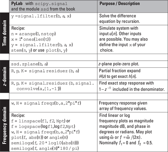
Figure 15-3: Working with LCC difference equations across domains by using PyLab.

Figure 15-3 parallels the content of Figure 15-2, so I simply point out differences in the content here:

In the time domain rows, you solve the difference equation exactly, using signal.lfilter(b,a,x).

In the z-domain rows, you can find the pole-zero plot of the system function H(z), using ssd.zplane(b,a), and the partial fraction expansion, using signal.residuez instead of signal.residue.

The frequency domain rows show you how to find the frequency response of a discrete-time system with signal.freqz(b,a,2*pi*f), where f is the frequency variable normalized by .

Mashing Domains in Real-World Cases

This section contains two examples that show how analysis and modeling across domains works. The examples include the time, frequency, and s- and z-domains. The first problem sticks to continuous-time, but the second one works across continuous- and discrete-time systems. A third example problem is available at www.dummies.com/extras/signalsandsystems.

Problem 1: Analog filter design with a twist

You’re given the task of designing an analog (continuous-time) filter to meet the amplitude response specifications shown in Figure 15-4. You also need to find the filter step response, determine the value of the peak overshoot, and time where the peak overshoot occurs.

The objective of the filter design is for the frequency response magnitude in dB () to pass through the unshaded region of the figure as frequency increases. The design requirements reduce to the passband and stopband critical frequencies fp and fs Hz and the passband and stopband attenuation levels Ap and As dB.

Additionally, the response characteristic is to be Butterworth, which means that the filter magnitude response and system function take this form:

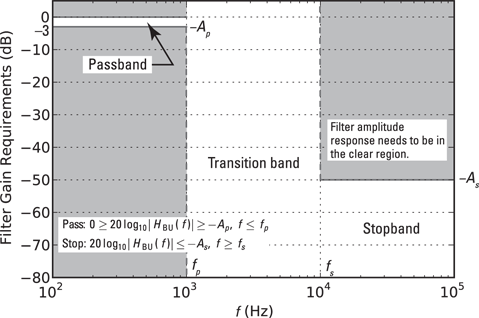
Figure 15-4: Analog low-pass filter design requirements.

Here, N is the filter order, is the passband 3 dB cutoff frequency of the filter, and the poles, located on a semicircle is the left-half s-plane, are given by .

This problem requires you to work in the frequency domain, the time domain, and perhaps the s-domain, depending on the solution approach you choose.

From the requirements, the filter frequency response has unity gain (0 dB) in the passband. The step response (a time-domain characterization) of the Butterworth filter is known to overshoot unity before finally settling to unity as .

To design the filter, you can use one of two approaches:

1. Work a solution by hand, using the Butterworth magnitude frequency response |HBU(f)| and the system function, HBU(s).

2. Use the filter design capabilities of the SciPy signal package.

I walk you through option two in the next section.

Finding the filter order and 3 dB cutoff frequency

Follow these steps to design the filter by using Python and SciPy to do the actual number crunching:

1. Find N and to meet the magnitude response requirements.

Use the SciPy function N,wc=signal.buttord(wp,ws,Ap,As,analog=1) and enter the filter design requirements, where wp and ws are the passband and stopband critical frequencies in rad/s and Ap and As are the passband and stopband attenuation levels (both sets of numbers come from Figure 15-4). The function returns the filter order N and the cutoff frequency wc in rad/s.

2. Synthesize the filter — find the coefficients of the LCC differential equation that realizes the desired system.

If finding circuit elements is the end game, you may go there immediately, using circuit synthesis formulas, which aren't described in this book. Call the SciPy function b,a=signal.butter(N,wc,analog=1) with the filter order and the cutoff frequency, and it returns the filter coefficients in arrays b and a.

3. Find the step response in exact mathematical form or via simulation.

Here’s how to use the Python tools with the given design requirements and then check the work by plotting the frequency response as an overlay to Figure 15-4. Note: You can do the same thing in MATLAB with almost the same syntax.

In [379]: N,wc =signal.buttord(2*pi*1e3,2*pi*10e3,3.0,

50,analog=1) # find filter order N

In [380]: N # filter order

Out[380]: 3

In [381]: wc # cutoff freq in rad/s

Out[381]: 9222.4701630595955

In [382]: b,a = signal.butter(N,wc,analog=1) # get coeffs.

In [383]: b

Out[383]: array([7.84407571e+11+0.j])

In [384]: real(a)

Out[384]: array([1.00000000e+00, 1.84449403e+04,

1.70107912e+08,7.84407571e+11])

The results of Line [379] tell you that the required filter order is N = 3 and the required filter cutoff frequency is 9,222.5 rad/s (). The filter coefficient sets are also included in the results.

I use the real() function to safely display the real part of the coefficients array a because I know the coefficients are real. How? The poles, denominator roots of HBU(s), are real or occur in complex conjugate pairs, ensuring that the denominator polynomial has real coefficients when multiplied out. The very small imaginary parts, which I want to ignore, are due to numerical precision errors.

Checking the final design frequency response

To check the design, use the frequency response recipe from Figure 15-2.

In [386]: f = logspace(2,5,500) # log frequency axis

In [387]: w,H = signal.freqs(b,a,2*pi*f)

In [388]: semilogx(f,20*log10(abs(H)),'g')

Figure 15-5 shows the plot of the final design magnitude response along with the original design requirements. I use the frequency-domain recipe from Figure 15-2 to create this design.

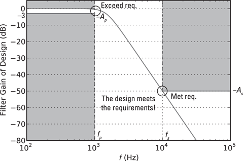
Figure 15-5: Magnitude frequency response of the final design meets the requirements.

Finding the step response from the filter coefficients

The most elegant approach to finding the step response from the filter coefficients is to find . The s-domain section of Figure 15-2 tells you how to complete the partial fraction expansion (PFE) numerically. You have the coefficient arrays for , so all you need to do is multiply the denominator polynomial by s. You can do this by hand or you can use a relationship between polynomial coefficients and sequence convolution.

When you multiply two polynomials, the coefficient arrays for each polynomial are convolved, as in sequence convolution (see Chapter 6).

Here, I work through the problem, using signal.convolve to perform polynomial multiplication in the denominator. To convince you that this really works, consider multiplication of the following two polynomials:

If you convolve the coefficients sets [1, 1, 1] and [1, 1] as arrays in Python, you get this output:

In [418]: signal.convolve([1,1,1],[1,1])

Out[418]: array([1, 2, 2, 1])

This agrees with the hand calculation. To find the PFE, plug the coefficients arrays b and convolve(a,[1,0]) into R,p,K = residue(b,a). The coefficients [1, 0] correspond to the s-domain polynomial s + 0.

In [420]: R,p,K = signal.residue(b,signal.convolve([1,0],a))

In [421]: R #(residues) scratch tiny numerical errors

Out[421]:

array([ 1.0000e+00 +2.3343e-16j, # residue 0, imag part 0

-1.0000e+00 +1.0695e-15j, # residue 1, imag part 0

1.08935e-15 -5.7735e-01j, # residue 2, real part 0

1.6081e-15 +5.7735e-01j]) # residue 3, real part 0

In [422]: p #(poles)

Out[422]:

array([ 0.0000 +0.0000e+00j, # pole 0

-9222.4702 -1.5454e-12j, # pole 1, imag part 0

-4611.2351 -7.9869e+03j, # pole 2

-4611.2351 +7.9869e+03j])# pole 3

In [423]: K #(from long division)

Out[423]: array([ 0.+0.j]) # proper rational, so no terms

I crossed out parts of Lines Out[421] and Out[422] to indicate that in absence of small numerical errors, the true values should be zero.

You have four poles: two real and one complex conjugate pair — a bit of a mess to work through, but it’s doable. Refer to the transform pair (see Chapter 13) to calculate the inverse transform for all four terms.

For the conjugate poles, the residues are also conjugates. This property always holds.

You can write the inverse transform of the conjugate pole terms as sines and cosines, using Euler’s formula and the cancellation of the imaginary parts in front of the cosine and real parts in front of the sine: , where . Putting it all together, you get .

Having this form is nice, but you still need to find the function maximum for and the maximum location. To do this, plot the function and observe the maximum.

A more direct approach is to use simulation via signal.lsim and the time-domain recipe from Figure 15-2. The system input is a step, so the simulation output will be the step response of Figure 15-6. From the simulated step response, you can calculate the peak overshoot numerically and see it in a plot. The IPython command line code is

In [425]: t = arange(0,0.002,1e-6) # step less than smallest time constant

In [426]: t,ys,x_state = signal.lsim((b,a),ones(len(t)),t)

In [428]: plot(t*1e3,ys)

Figure 15-6: Third-order Butterworth filter step response.

Using the time array t and the step response array ys, you can use the max() and find() functions to complete the task:

In [436]: max(real(ys)) # real to clear num. errors

Out[436]: 1.0814651457627822 # peak overshoot is8.14%

In [437]: find(real(ys)== max(real(ys)))

Out[437]: array([534]) # find peak to be at index 534

In [439]: t[534]*1e3 # time at index 534 in ms

Out[439]: 0.5339

Problem 2: Solving the DAC ZOH droop problem in the z-domain

The zero-order-hold (ZOH), that’s inherent in many digital-to-analog converters (DACs), holds the analog output constant between samples. The action of the ZOH introduces frequency droop, a roll off of the effective DAC frequency response on the frequency interval zero to one-half the sampling rate fs, in reconstructing from . Two possible responses are to

Apply an inverse sinc function shaping filter in the continuous-time domain.

Correct for the droop before the signal emerges from the DAC.

The system block diagram is shown in Figure 15-7.

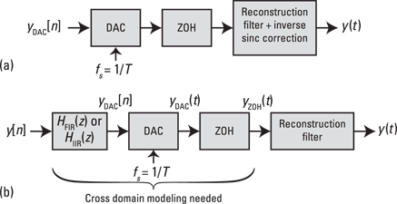
Figure 15-7: DAC ZOH droop compensation system block diagram: pure analog filter solution (a) and hybrid discrete-time and analog solution (b).

Imagine that a senior engineer asks you to investigate the effectiveness of the simple infinite impulse response (IIR) and finite impulse response (FIR) digital filters as a way to mitigate ZOH frequency droop. You need to verify just how well these filters really work. The filter system functions are

To solve this problem, you need to use the frequency-domain relationship from the discrete- to continuous-time domains. As revealed in Figure 15-1, the relationship, relative to the notation of Figure 15-7, is for . You can assume that the analog reconstruction filter removes signal spectra beyond fs/2.

The frequency response of interest turns out to be the cascade of and . Follow these steps to justify this outcome:

1. Let . From the convolution theorem for frequency spectra in the discrete-time domain, get .

2. Use the discrete to continuous spectra relationship to discover that the output side of the DAC is .

3. Use the convolution theorem for frequency spectra in the continuous-time domain to push the DAC output spectra through the ZOH filter:

The cascade result is now established.

To view the equivalent frequency response for this problem in the discrete-time domain, you just need to change variables according to the sampling theory: , where and T = 1/fs. Rearranging the variables in the cascade result viewed from the discrete-time domain perspective is . The ZOH frequency response is

Putting the pieces together and considering only the magnitude response reveals this equation:

To verify the performance, evaluate the sinc function and the FIR responses by using the SciPy signal.freqz() function approach of the frequency domain recipe in Figure 15-3. Check out the results in Figure 15-8.

In [393]: w = linspace(0,pi,400)

In [394]: H_ZOH_T = sinc(w/(2*pi))

In [395]: w,H_FIR = signal.freqz(array([-1, 18,-1])/16.,1,w)

In [396]: w,H_IIR = signal.freqz([-9/8.],[1, 1/8.],w)

In [402]: plot(w/(2*pi),20*log10(abs(H_ZOH_T)))

In [403]: # other plot cammand lines similar

In [412]: plot(w/(2*pi),20*log10(abs(H_FIR)*abs(H_ZOH_T)))

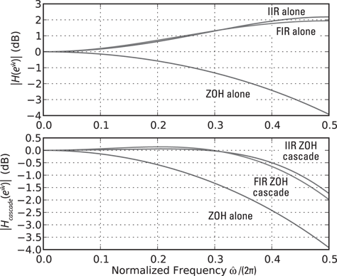
Figure 15-8: The result of placing a simple FIR or IIR filter ahead of a DAC with ZOH to provide droop compensation.

I think these results are quite impressive for such simple correction filters. The goal is to get flatness that’s near 0 dB from 0 to rad/sample (0 to 0.5 normalized). The response is flat to within 0.5 dB out to 0.4 rad/sample for the IIR filter; it’s a little worse for the FIR filter.

Find an additional problem that shows you how to take the RC low-pass filter to the z-domain at www.dummies.com/extras/signalsandsystems.