
Chapter 4
Discrete-Time Signals and Systems
In This Chapter
![]() Considering the different types of discrete-time signals
Considering the different types of discrete-time signals
![]() Modifying discrete-time sequences
Modifying discrete-time sequences
![]() Working with real signals in discrete-time
Working with real signals in discrete-time
![]() Checking out discrete-time systems
Checking out discrete-time systems
We live in a continuous-time/analog world; but people increasingly use computers to process continuous signals in the discrete-time domain. From a math standpoint, discrete-time signals and systems can stand alone — independent of their continuous-time counterparts — but that isn’t the intent of this chapter. Instead, I want to show you how discrete-time signals and systems get the job done in a way that’s parallel to the continuous-time description in Chapter 3.
A great deal of innovation takes place in discrete-time signals and systems. High-performance computer hardware combined with sophisticated algorithms offer a lot of flexibility and capability in manipulating discrete-time signals. Computers can carry out realistic simulations, which is a huge help when studying and designing discrete-time signals and systems.
Continuous- and discrete-time signals have a lot in common. In this chapter, I describe how to classify signals and systems, move signals around the time axis, and plot signals by using software. Also, because discrete-time signals often begin in the continuous-time domain, I point out some details of converting signals late in the chapter.
Exploring Signal Types
Like the continuous-time signals, discrete-time signals can be exponential or sinusoidal and have special sequences. The unit sample sequence and the unit step sequence are special signals of interest in discrete-time. All these signals have continuous-time counterparts, but singularity signals (covered in Chapter 3) appear in continuous-time only.
Note: Discrete-time signals are really just sequences. The independent variable is an integer, so no in-between values exist. A bracket surrounds the time variable for discrete-time signals and systems — as in x[n] versus the x(t) used for continuous-time. The values that discrete-time signals take on are concrete; you don’t need to worry about limits.
Exponential and sinusoidal signals
Exponential signals and real and complex sinusoids are important types of signals in the discrete-time world. Sinusoids, both real and complex, are firmly rooted in discrete-time signal model and applications. Signals composed of sinusoids can represent communication waveforms and the basis for Fourier spectral analysis, both the discrete-time Fourier transform (described in Chapter 11) and the discrete Fourier transform and fast Fourier transform (Chapter 12).
The exponential sequence ![]() is a versatile signal. By letting
is a versatile signal. By letting ![]() and
and ![]() be complex quantities in general, this signal alone can represent a real exponential, a complex sinusoid, a real sinusoid, and exponentially damped complex and real sinusoids. For definitions of these terms, flip to Chapter 3.
be complex quantities in general, this signal alone can represent a real exponential, a complex sinusoid, a real sinusoid, and exponentially damped complex and real sinusoids. For definitions of these terms, flip to Chapter 3.
Figure 4-1 shows stem plots of three variations of the general exponential sequence.
In the remaining material, let ![]() and
and ![]() .
.
The real exponential is formed when ![]() . A unit step sequence (described later in this section) is frequently included. The result is
. A unit step sequence (described later in this section) is frequently included. The result is ![]() .
.
If ![]() , the sequence is decreasing. Without any assumptions about
, the sequence is decreasing. Without any assumptions about ![]() and
and ![]() , you get a full complex exponential sequence:
, you get a full complex exponential sequence:
![]()
The envelope may be growing, constant, or decaying, depending on ![]() , respectively. For
, respectively. For ![]() , you have a complex sinusoidal sequence:
, you have a complex sinusoidal sequence:
![]()
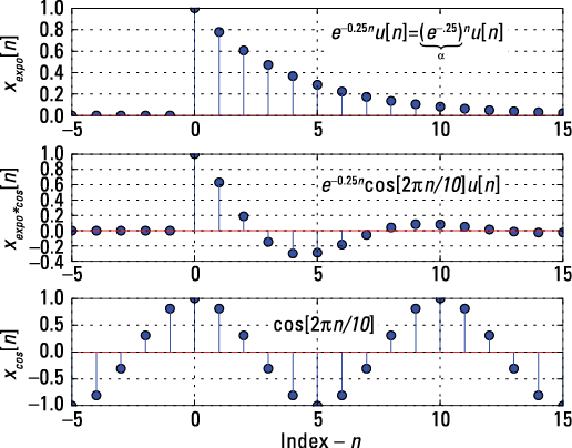
Figure 4-1: Stem plots of a real exponential ![]()
![]() , an exponentially damped cosine
, an exponentially damped cosine ![]()
![]() , and a cosine sequence
, and a cosine sequence ![]() ;
; ![]() in all three plots.
in all three plots.
In the discrete-time domain, complex sinusoids are common and practical, because computers can process complex signals by just adding a second signal path in software/firmware. The continuous-time complex sinusoid found in Chapter 3 requires a second wired path, increasing the complexity considerably.
Finally, if you consider just the real part of x[n], with ![]() , you get the real sinusoid
, you get the real sinusoid ![]() .
.
Just as in the case of the continuous-time sinusoid, the definition has three parameters: The amplitude A and phase ![]() carry over from the continuous-time case; the frequency parameter doesn’t. What gives?
carry over from the continuous-time case; the frequency parameter doesn’t. What gives?
In the continuous-time case, the cosine argument (less the phase) is ![]() . Tracking the units is important here. The radian frequency
. Tracking the units is important here. The radian frequency ![]() has units radians/second (
has units radians/second (![]() has units of hertz), so the cosine argument has units of radians, which is expected. But in the discrete-time case, the cosine argument (again less the phase) is
has units of hertz), so the cosine argument has units of radians, which is expected. But in the discrete-time case, the cosine argument (again less the phase) is ![]() . The time axis n has units of samples, so it must be that
. The time axis n has units of samples, so it must be that ![]() has units of radians/sample. It’s now clear that
has units of radians/sample. It’s now clear that ![]() aren’t the same quantity!
aren’t the same quantity!
But there’s more to the story. In practice, discrete-time signals come about by uniform sampling along the continuous-time axis t. Uniform sampling means ![]() , where T is the sample spacing and
, where T is the sample spacing and ![]() is the sampling rate in hertz (actually, samples per second). When a continuous-time sinusoid is sampled at rate
is the sampling rate in hertz (actually, samples per second). When a continuous-time sinusoid is sampled at rate ![]() ,
, ![]() so it must be that
so it must be that ![]() .
.
 A fundamental result of uniform sampling is that discrete-time frequencies and continuous-time frequencies are related by this equation:
![]()
This result holds so long as ![]() , a condition that follows from low-pass sampling theory. When the condition isn’t met, aliasing occurs. The continuous-time frequency won’t be properly represented in the discrete-time domain; it will be aliased — or moved to a new frequency location that’s related to the original frequency and the sampling frequency. See Chapter 10 for more details on sampling theory and aliasing.
, a condition that follows from low-pass sampling theory. When the condition isn’t met, aliasing occurs. The continuous-time frequency won’t be properly represented in the discrete-time domain; it will be aliased — or moved to a new frequency location that’s related to the original frequency and the sampling frequency. See Chapter 10 for more details on sampling theory and aliasing.
Special signals
The signals I consider in this section are defined piecewise, meaning they take on different functional values depending on a specified time or sequence interval. The first signal I consider, the unit impulse, has only one nonzero value. Most of the special signals are defined over an interval of values (more than just a point).
The unit impulse sequence
The unit impulse, or unit sample, sequence is defined as
![]()
This definition is clean, as opposed to the continuous-time unit impulse, ![]() , defined in Chapter 3. Any sequence can be expressed as a linear combination of time-shifted impulses:
, defined in Chapter 3. Any sequence can be expressed as a linear combination of time-shifted impulses:
![]()
This representation of x[n] is important in the development of the convolution sum formula in Chapter 6. Note that time or sequence shifting of ![]() — that is,
— that is, ![]() — moves the impulse location to
— moves the impulse location to ![]() . Why? The function turns on when
. Why? The function turns on when ![]() because n = k is the only time that
because n = k is the only time that ![]() .
.
The unit step sequence
The unit step sequence is defined as
![]()
Note that unlike the continuous-time version, u[n] is precisely defined at ![]() . The unit step and unit impulse sequences are related through these relationships:
. The unit step and unit impulse sequences are related through these relationships:

As you can see, the unit step sequence is simply a sum of shifted unit impulses that repeats infinitely to the right, starting with n = 0. This is just one example of how any sequence can be written as a linear combination of shifted impulses — pretty awesome!
 Example 4-1: Use the unit step sequence to create a rectangular pulse sequence of length L samples. The pulse is to turn on at
 ![]() and stay on for L total samples.
and stay on for L total samples.
The solution is quite simple, ![]() , but watch the details. When
, but watch the details. When ![]() , the second unit step turns on and begins to subtract +1s from the first step. The first nonzero point occurs at
, the second unit step turns on and begins to subtract +1s from the first step. The first nonzero point occurs at ![]() , and the last nonzero point occurs at
, and the last nonzero point occurs at ![]() . So how many nonzero points are there?
. So how many nonzero points are there?
The total number of points in the pulse is ![]() , as desired. Figure 4-2 shows the formation of the rectangular pulse sequence for
, as desired. Figure 4-2 shows the formation of the rectangular pulse sequence for ![]() .
.
The Python support function dstep(), found in ssd.py, generates a unit step sequence that's used to create a ten sample pulse sequence:
In [10]: import ssd # at the start of the session
In [11]: n = arange(-5,15+1) # create time axis n
In [13]: stem(n,ssd.dstep(n))# plot u[n]
In [18]: stem(n,ssd.dstep(n-10))# plot u[n-10]
In [23]: stem(n,ssd.dstep(n)-ssd.dstep(n-10))# difference

Figure 4-2: Formation of a rectangular pulse sequence from two unit step sequences.
Window functions
Signals pass through windows just as light passes through the glass in your house or office; how illuminating! You may want to think of windows as the rectangular pulses of discrete-time. Just keep in mind that windows may not always be rectangular; sometimes they’re tapered. Nevertheless, these discrete-time signals are more than academic; they’re shapes used in real applications.
In one application, you use a window function w[n] to multiply or weight a signal of interest, thereby forming a windowed sequence: ![]() .
.
Window functions are also used in digital filter design. The L sample rectangular pulse of Example 4-1 shows the natural windowing that occurs when capturing an L sample chunk of signal x[n] by multiplying x[n] by w[n].
In general, the sample values of a window function smoothly taper from unity near the center of the window to zero at each end. The rectangular window, just like the rectangle pulse, is a constant value from end to end and thus provides no tapering. In spectral analysis, a tapered window allows a weak signal to be discerned spectrally from a strong one. Windowing in a digital filter makes it harder for unwanted signals to leak through the filter.
To fully appreciate windowing, you need to understand frequency-domain analysis, the subject of Part III. Specifically, I describe spectral analysis of discrete-time signals in Chapter 12.
Example 4-2: The signal package, specifically, signal.windows, of the Python library SciPy contains more than ten window functions! As a specific example, the Hann (also known as the Hanning) window is defined as follows:
![]()
The IPython command line input, which calls the hann(L) window function to generate a 50 sample window is
In [138]: import scipy.signal as signal
In [139]: w_hann = signal.windows.hann(50)
Pulse shapes
In digital communication, a pulse shape, p[n], creates a digital communication waveform that’s bandwidth or spectrally efficient. A mathematical representation of a digital communication signal/waveform is the sequence
![]()
where the ![]() are
are ![]() data bits (think 0s and 1s), and
data bits (think 0s and 1s), and ![]() is the duration of each data bit in samples.
is the duration of each data bit in samples.
Popular pulse shapes used for digital communications include the rectangle (RECT), half-sine (HC), the raised cosine (RC), and the square-root raised cosine (SRC or RRC). You can find the definitions of these pulse shapes and more detailed information on their use in real systems in a digital communications case study at www.dummies.com/extras/signalsandsystems.
The Python function NRZ_bits() generates the digital communications signal x[n]. The function returns x, p, and data, which are the communications waveform, the pulse shape, and the data bits encoded into the waveform. Find details on the capabilities of this and supporting functions at ssd.py.
Surveying Signal Classifications in the Discrete-Time World
Like their continuous-time counterparts, discrete-time signals may be deterministic or random, periodic or aperiodic, power or energy, and even or odd. Discrete-time also has special sequences as well as exponential and sinusoidal signals. I explain the details of these signal types and point out how they compare to continuous-time signals in the following sections.
Deterministic and random signals
Discrete-time signals may be deterministic or random. Discrete signal x[n] is deterministic if it’s a completely specified function of time, n. As a simple example, consider the following finite sequence:
![]()
The symbol ![]() is a timing marker denoting where
is a timing marker denoting where ![]() . Outside the interval shown, I assume the sequence is 0.
. Outside the interval shown, I assume the sequence is 0.
The customary way of plotting a discrete-time signal is by using a stem plot, which locates a vertical line at each n value from zero to the sequence value x[n]; a stem plot also includes a marker such as a filled circle. PyLab and other similar software tools provide support for such plots.
 To create the stem plot, using the sequence definition for x[n], create a vector
 x (NumPy ndarray) to hold the signal values and a vector n to hold the time index values. The time index values consist of values from –4 ≤ n ≤ 7. These values correspond to each value of the sequence x[n], with reference taken to the timing marker.
In [466]: n = arange(-4,7+1) # creates -4<=n<=7
In [467]: x = array([0,2,2,2,1,0,-1,-1,-3,1,1,0])
In [468]: stem(n,x) # create the stem plot
Figure 4-3 illustrates this stem plot.
The stem plot is ideal here because connecting the points isn't really appropriate for a signal that's defined only at integer values. PyLab's stem() function, which creates the stem plot, is quite flexible by allowing for different colors and stem head symbols (to see how, type stem? at the IPython command prompt).
 A random signal, w[n], takes on unpredictable values according to some probability distribution. A computer or state machine (a mathematical model of computation) is typically nearby in the case of discrete-time signals, so you can generate w[n] by using a software-based random number generator. Technically speaking, the sequence is only pseudo-random, because computer-generated random numbers eventually repeat. Still, you can get a good approximation of a random signal in practice. Python, in particular NumPy, provides an excellent random number library.
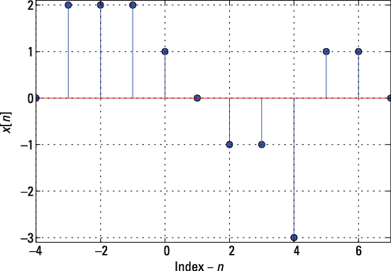
Figure 4-3: A stem plot of the deterministic signal x[n].
At the command prompt, type In [5]: random? for a helpful listing of the distribution types available.
Gaussian and uniform distributed random sequences are common choices in signal modeling; for example:
In [6]: randn(4) # 4 numbers, mean = 0, variance = 1
Out[6]:
array([-1.509427, -0.779072, 0.643483, -1.020021])
In [7]: uniform(0,1,4) # 4 numbers uniform on (0, 1)
Out[7]:
array([0.114319, 0.415064, 0.330576, 0.266975])
Periodic and aperiodic
Sinusoidal sequences behave differently in discrete-time situations; they’re not always periodic here as they are in the world of continuous-time.
A discrete-time signal, x[n], is periodic with period N0, for the smallest integer ![]() resulting in
resulting in ![]() . If
. If ![]() can’t be found, the signal is aperiodic.
can’t be found, the signal is aperiodic.
Example 4-3: Using IPython, you can create a short sequence, ![]() , of ten samples and then embed this sequence in a larger one, using the
, of ten samples and then embed this sequence in a larger one, using the mod()
function. Define ![]() . A second sequence,
. A second sequence, ![]() is plotted.
is plotted.
Here is the Python code for plotting:
In [474]: n = arange(0,31) # n-axis for plotting
In [475]: x_p = array([1,1,-1,0,2,0,0,0,0,0]) # one period
In [476]: x_10 = x_p[mod(n,10)] # 3+ periods
In [477]: subplot(211); stem(n,x_10) # plot per. 10 seq.
In [478]: subplot(212); stem(n,cos(6*n/10.) # aper. cos
The two sequences are shown in Figure 4-4 as subplots.
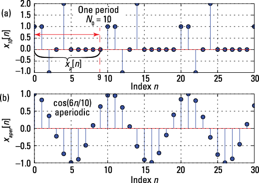
Figure 4-4: A stem plot of the periodic sequence ![]() , created from
, created from ![]() (a) and a cosine sequence that by inspection isn’t periodic (b).
(a) and a cosine sequence that by inspection isn’t periodic (b).
Note the signal ![]() by itself is aperiodic, because it’s an isolated sequence of nonzero values. The cosine sequence appears to be periodic.
by itself is aperiodic, because it’s an isolated sequence of nonzero values. The cosine sequence appears to be periodic.
To make a sinusoidal sequence periodic, the following expressions must be equal:
![]()
Cosine is a ![]() function, so for the equality to hold, the following must be true:
function, so for the equality to hold, the following must be true:
![]()
Rearranging, you have
![]()
The conclusion is that a sinusoidal sequence can be periodic only if ![]() is a rational number multiple of
is a rational number multiple of ![]() . The smallest
. The smallest ![]() satisfying the equation is the period of the sinusoid.
satisfying the equation is the period of the sinusoid.
For multiple sinusoids to be periodic, you need to find a common ![]() that works for all the sinusoids together.
that works for all the sinusoids together.
In Example 4-6, ![]() . This means that 3/(10π) is irrational by virtue of the π in the denominator.
. This means that 3/(10π) is irrational by virtue of the π in the denominator.
Also, because sine/cosine are ![]() functions, the frequencies
functions, the frequencies ![]() and
and ![]() are indistinguishable, meaning they produce the same functional values. To be clear for m = 1,
are indistinguishable, meaning they produce the same functional values. To be clear for m = 1, ![]()
![]() because cosine is a
because cosine is a ![]() function. This result is independent of the sinusoidal sequence being periodic. The fundamental interval is often taken as
function. This result is independent of the sinusoidal sequence being periodic. The fundamental interval is often taken as ![]() .
.
For the special case of a sinusoid having period ![]() , the distinguishable frequencies are the
, the distinguishable frequencies are the ![]() values:
values:
![]()
Distinguishable frequencies are distinct from all other frequencies that result in a sinusoidal sequence having period N0 and lie on the fundamental frequency interval.
Example 4-4: Consider the signal ![]() . Find the period of
. Find the period of ![]() , and calculate the power,
, and calculate the power, ![]() . The sinusoids have frequency
. The sinusoids have frequency ![]() . They’re both periodic with periods of 10 and 21, respectively. The least common multiple is 210, so the overall period is
. They’re both periodic with periods of 10 and 21, respectively. The least common multiple is 210, so the overall period is ![]() .
.
For multiple sinusoidal sequences, the following is true:
![]()
For continuous-time sinusoid ![]() , you can show that increasing
, you can show that increasing ![]() increases the oscillation rate (number of cycles per second). For
increases the oscillation rate (number of cycles per second). For ![]() , the oscillation increases while
, the oscillation increases while ![]() , and then it decreases back to 0 for
, and then it decreases back to 0 for ![]() .
.
The oscillation rate increase and decrease property for the discrete-time sinusoid is verified in Figure 4-5.
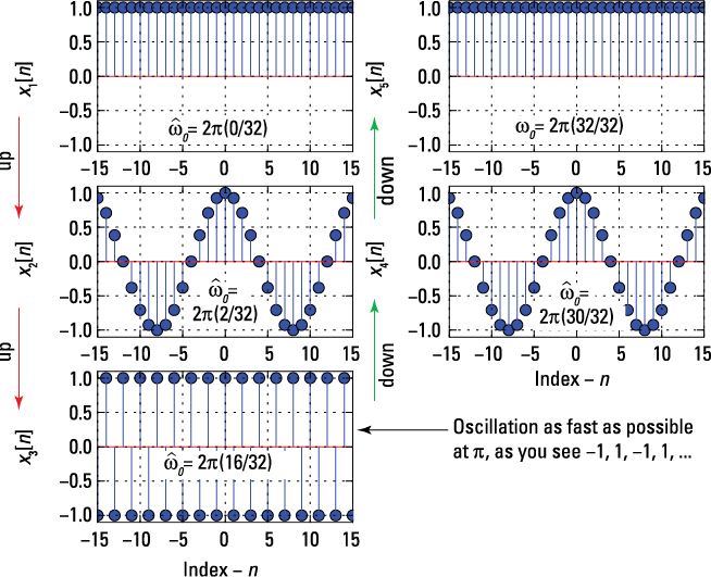
Figure 4-5: Plots of ![]() showing increasing oscillation rate as
showing increasing oscillation rate as ![]() approaches
approaches ![]() then symmetrically decreasing as
then symmetrically decreasing as ![]() approaches
approaches ![]() .
.
Recognizing energy and power signals
In discrete-time, a signal can be classified as being energy, power, or neither. Here are the expressions for discrete-signal energy, Ex, and power, Px:

In the case of a continuous-time signal, the units for power and energy are watts (W) and joules (J). For the discrete-time case, the units don’t formally apply unless you find x[n] by sampling a continuous-time signal — that is, ![]() . The signal x[n] is
. The signal x[n] is
![]() An energy signal if
An energy signal if ![]() and
and ![]()
![]() A power signal if
A power signal if ![]() and
and ![]()
![]() Neither power nor energy if both
Neither power nor energy if both ![]() and
and ![]() go to infinity
go to infinity
An aperiodic signal of finite duration is a good example of an energy signal, and a sinusoidal signal (sequence) is a good example of a power signal. See Chapter 3 for the definition of aperiodic signal.
Example 4-5: To find the energy in the signal ![]() , plug the values into the energy formula:
, plug the values into the energy formula:
![]()
Example 4-6: Find the power in the sinusoidal signal ![]() , where
, where ![]() is the sinusoidal discrete-time frequency in radians per sample and
is the sinusoidal discrete-time frequency in radians per sample and ![]() .
.
If x[n] is periodic, you can take a shortcut and apply the definition over just one periodic: ![]() . You must use the full definition when x[n] is aperiodic, so you calculate the power as follows:
. You must use the full definition when x[n] is aperiodic, so you calculate the power as follows:

Intuitively, the second term of the third line reduces to 0 for large N. The formula for power in a discrete-time sinusoid then becomes ![]() . (The same result occurs in Chapter 3 for the continuous-time sinusoid.) The path you take to get the discrete-time results is different because of the summation instead of the integral, but the results are consistent with the continuous-time case.
. (The same result occurs in Chapter 3 for the continuous-time sinusoid.) The path you take to get the discrete-time results is different because of the summation instead of the integral, but the results are consistent with the continuous-time case.
Computer Processing: Capturing Real Signals in Discrete-Time
Example 4-7: For speech analysis, you can use a tool, such as Python with PyLab, to analyze real signals. By real, I mean a signal captured from the continuous-time domain. In this example, I assume you connect a microphone to the audio input of your computer and capture in wav file format the utterance of the two-syllable word zero twice. Perhaps you need to design a speech recognition system for “zero-zero.” Figure 4-6 shows the system block diagram.
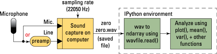
Figure 4-6: Block of audio capture into IPython.
Depending on the audio inputs on your computer, you may need to add a microphone preamp. In the following sections, I explain the wav file you capture and show how you can use Python to find the signal energy and average power in discrete-time.
Capturing and reading a wav file
Using readily available recording software, set the sampling rate to ![]() kHz, which is 22,050 samples per second. The samples are spaced by the sampling period
kHz, which is 22,050 samples per second. The samples are spaced by the sampling period ![]() . Save the recorded sound in the file
. Save the recorded sound in the file zerozero.wav. The module ssd.py contains functions for reading and writing wav files. The command for reading a wav file is:
In [481]: fs, zerozero_wav = ssd.wave_read('zerozero.wav')
Note that wavfile.read() returns the sampling rate fs and the NumPy ndarray zerozero_wav, ready for plotting and further analysis.
You can discover a little about the capture by using some of the properties associated with fs and zerozero_wav:
In [400]: zerozero_wav.dtype
Out[480]: dtype('float64')
In [480]: zerozero_wav.shape
Out[480]: (76024, 2)
In [481]: fs
Out[481]: 22050
The function scales the sample values from 16-bit signed integers to 64-bit floats (see Line [480]). Line [481] tells you that the input array is composed of two columns and 76,024 rows (samples). There are two columns because the recording was made in stereo. I used a single channel microphone so identical signal values are found in each column. The syntax zerozero_wav[:,0] extracts just column zero. If you divide the number of samples by the sampling rate, you get the duration of the recording: N/fs = 76,024/22,050 = 3.45 s.
The signal is discrete-time, but a large number of points occur, so plot() is preferred over stem() in this case.
Figure 4-7 shows a subplot() array containing two views of the signal. The IPython command line code (abbreviated) is
In [488]: plot(zerozero_wav[:,0])
In [492]: plot(zerozero_wav[:,0])
In [495]: axis([12000, 22000, -0.3, 0.3]) # zoom axis
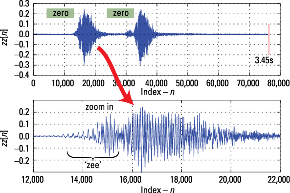
Figure 4-7: A subplot of the speech file zerozero.wav.
Figure 4-7 shows that the two zero utterances aren’t all that similar. Surprised? The z in zero is distinctive in the zoom plot. Do you think a speech signal is deterministic or random? Random! In the context of this single data record, you can view the signal as a deterministic waveform. Because the signal has only two segments, you can also classify this as an energy signal.
If these two segments are part of a much longer speech record, you can use them to estimate the average power of the entire record.
Finding the signal energy
To calculate the signal energy of the two zeros recorded at 22,050 samples per second (sps), I form the sum of the squared sample values (Line [500]):
In [500]: E_zz = sum(zerozero_wav[:,0]**2) #sq & sum samps
In [541]: E_zz
Out[541]: 92.6137 # the signal energy
You can calculate the signal average value or mean by using mean() and the variance, essentially the signal power, by using var().
Want to know how indexing and slicing work in Python? Suppose x is a ![]() ndarray. In Python, array indexes start at
ndarray. In Python, array indexes start at 0 and end at N–1 (len(vec)-1). The first element is x[0], and the last element is x[–1] because a negative index means to count backward from the end; that is, x[–2] = x[len(x)–2]. Slicing, which involves the use of :, allows you to select a contiguous interval anywhere from 0 to N–1. So x[2:5] returns the elements 2 to 5–1, x[:5] returns elements 0 to 4, x[2:] returns elements 2 to N–1, and x[:] returns all the elements. In a two-dimensional array, indexing and slicing works the same, except you have two indexes to play with, as in x[i,j].
Classifying Systems in Discrete-Time
You can classify discrete-time systems based on their properties. Here, I point out how to check a discrete-time system for the following properties: linear/nonlinear, time-invariant/time-varying, causal/non-causal, memory/memoryless, and bounded-input bounded-output (BIBO) stability. (See Chapter 3 for a description of the mathematical properties of these classifications.)
Consider a generic discrete-time system ![]() that’s defined as an operator that maps the input sequence to the output sequence. Figure 4-8 shows a block diagram representation of the system.
that’s defined as an operator that maps the input sequence to the output sequence. Figure 4-8 shows a block diagram representation of the system.
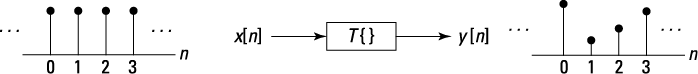
Figure 4-8: Discrete-time system block diagram definition.
Checking linearity
A system is linear if superposition holds. So, if
![]()
and a and b arbitrary constants
![]()
then the system is linear.
For K signals with ![]() , you can write:
, you can write:
![]()
If superposition doesn’t hold, the system is nonlinear.
Investigating time invariance
A system is time-invariant if properties or characteristics of the system don’t change with the time index. A mathematical statement of this is that given ![]() and any sequence offset
and any sequence offset ![]() , the time-shifted input
, the time-shifted input ![]() must produce system output
must produce system output ![]() .
.
A system that doesn’t obey this property is said to be time-varying. In the continuous-time domain, time-varying behavior can be due to uncontrollables, such as environmental conditions like temperature and/or component aging. In the discrete-time domain, an adaptive filter with time-varying attributes can optimize overall system performance. Cellular phone systems make use of this today. The channel between you and the base station changes as you move, so your handset adapts to the environment by changing system attributes. Welcome to the world of adaptive signal processing!
Looking into causality
The mathematical definition of causality states that a system is causal if all output values, ![]() , depend only on input values
, depend only on input values ![]() for
for ![]() . Another way of saying this is the present output depends only on past and present input values.
. Another way of saying this is the present output depends only on past and present input values.
A system is causal, or nonanticipative, if it doesn’t anticipate the arrival of the signal at the input. Non-causal systems can predict the future! For discrete-time systems, you’re more likely to talk about non-causal systems. In discrete-time signal processing, a signal may be stored in a file and processed in such a way that non-causal operations are used.
What’s the trick? Well, because the signal is stored in advance, the non-causal system has access to future values of the signal. The operations only appear non-causal. You can’t predict the future here, but in discrete-time signal processing, you can pretend that you can.
Figuring out memory
A system is memoryless if each output y[n] depends only on the present input x[n]. A memoryless system is always causal because there’s no chance that values other than the present input will be used for the present output. A causal system, however, doesn’t have to be memoryless. A causal system can use past values of the input to form the output. This puts memory into the system.
Checking system properties
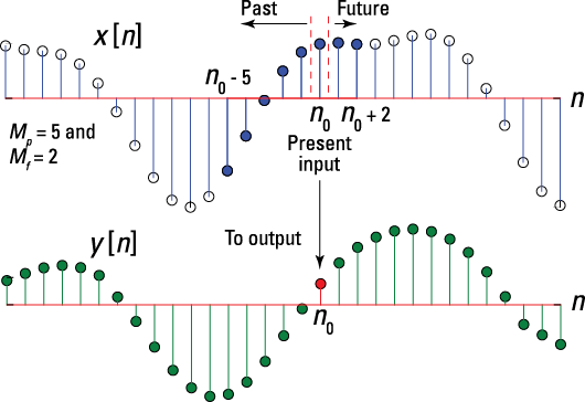
To get a firmer grip on the discrete-time version of these five system properties, consider the moving average (MA) system, which is defined as
![]()
With this system, the present output is the average (by virtue of the scale factor ![]() of the present input along with
of the present input along with ![]() past inputs and
past inputs and ![]() future inputs. Investors use moving averages. Only past values can be used to guide your next stock purchase. A graphical depiction of the MA system for
future inputs. Investors use moving averages. Only past values can be used to guide your next stock purchase. A graphical depiction of the MA system for ![]() is shown in the figure.
is shown in the figure.
Run through the five properties to see where this systems stands:
![]() Linearity: The system is linear because the output is a linear combination of
Linearity: The system is linear because the output is a linear combination of ![]() inputs.
inputs.
![]() Time invariance: The system is time-invariant because the system coefficients (the scale factor applied to each
Time invariance: The system is time-invariant because the system coefficients (the scale factor applied to each ![]() term) are constant.
term) are constant.
![]() Causality: The system isn’t causal as long as
Causality: The system isn’t causal as long as ![]() (see the figure).
(see the figure).
![]() Memory: The system isn’t memoryless if
Memory: The system isn’t memoryless if ![]() and/or
and/or ![]() .
.
![]() BIBO stability: The system is BIBO stable because the system coefficients are finite. To be more precise mathematically, I start with
BIBO stability: The system is BIBO stable because the system coefficients are finite. To be more precise mathematically, I start with ![]() and write
and write

The last term of the first line is due to the triangle inequality, which states that ![]() , for any x and y.
, for any x and y.
Testing for BIBO stability
A system is said to be bounded-input bounded-output (BIBO) stable if and only if every bounded input produces a bounded output. In other words, the signal x[n] (which may be the input or output) is bounded if some constant ![]() exists, such that
exists, such that ![]() for all values of n.
for all values of n.
 A challenge associated with this property is to show the property holds for any bounded input. Any is a lot of cases to test and requires some proof-writing skills.
Example 4-8: Consider the system ![]() . Run through the five properties to see where this system stands.
. Run through the five properties to see where this system stands.
![]() Linearity: The system isn’t linear because
Linearity: The system isn’t linear because

Why? From left to right, ![]() .
.
![]() Time invariance: The system isn’t time-invariant because the system coefficient
Time invariance: The system isn’t time-invariant because the system coefficient ![]() is time-varying. For
is time-varying. For ![]() , it’s 0, and for
, it’s 0, and for ![]() , it’s 1.
, it’s 1.
![]() Causality: The system is causal. No way, you say! The system term
Causality: The system is causal. No way, you say! The system term ![]() does turn on before
does turn on before ![]() , but this is a system property, not a future value of the input. Only past and present values of the input form each and every output. The time-varying bias term is out of the picture.
, but this is a system property, not a future value of the input. Only past and present values of the input form each and every output. The time-varying bias term is out of the picture.
![]() Memory: The system isn’t memoryless because the past input
Memory: The system isn’t memoryless because the past input ![]() forms the present output.
forms the present output.
![]() BIBO stability: The system is BIBO stable because the system coefficients are finite.
BIBO stability: The system is BIBO stable because the system coefficients are finite.
Interfacing to the analog world
The core building blocks for going from the analog (continuous-time) domain to the discrete-time domain and back are two mixed-signal subsystems. The analog-to-digital converter (ADC) and the digital-to-analogconverter (DAC) perform these functions. The term mixed signal denotes that the electronic circuit design of these subsystems involves both analog and digital circuit design. I provide additional details in Chapter 10, where I describe sampling theory.
The top-level model of the ADC and DAC interfaces to the discrete-time domain are shown in the figure .
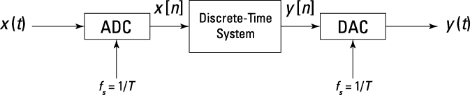
A sampling rate of ![]() samples per second (sps) is shown. This means that
samples per second (sps) is shown. This means that ![]() and
and ![]() , with interpolation of the y[n] values is used to create values for y(t) between the sample values. As long as the frequency content of x(t) is less than
, with interpolation of the y[n] values is used to create values for y(t) between the sample values. As long as the frequency content of x(t) is less than ![]() , you can also say that
, you can also say that ![]() . In practice, the discrete-time system modifies x[n] to suit your needs, so y(t) differs from x(t), but the difference is a good thing.
. In practice, the discrete-time system modifies x[n] to suit your needs, so y(t) differs from x(t), but the difference is a good thing.
The back half of the figure is similar to what goes on when you listen to MP3 or iPod music. Stereo audio samples from a CD or other digital music source having a nominal sampling rate of 44.1 ksps, are compressed 11:1 using what is known as perceptual coding. The compression reduces the memory needed to store the music and also the bandwidth needed for streaming over the Internet. Following decompression, the samples are further manipulated in some discrete-time system. The sampling rate is likely increased to 48 ksps, 96 ksps, or as high as 192 ksps. The DAC steps in, and you’re able to hear beautiful music.