Thermal Resistance and Board Construction

Switching power supplies dissipate much less than linear regulators as explained in Chapter 1. But they do. In Chapter 6, we saw the importance of lowering temperatures for maximizing reliability and life. We have learned of different ways to improve efficiency of switching power supplies, including the use of synchronous regulators as discussed in Chapter 9. But eventually, despite all our best efforts, there will be some dissipation still remaining. Most of this heat will be lost in the semiconductors, but some of it will be lost in the inductors too. Especially in AC–DC power supplies, a good deal of heat will also be lost in the EMI filter. In flyback power supplies, we typically need to parallel several output caps, to lower the effective ESR, and thereby lower the heat generated inside C_O. The zener clamp also gets very hot. With all these effects, not to mention some components heating up others in their vicinity, a final qualification stage for any commercial power supply will involve knowing the temperatures of each and every component on the board (usually by connecting hundreds of thermocouples if necessary) and calculating their temperature stress factors to ensure they are all being operated at typically better than at least 80% of their max temperature ratings.

The relationship between the dissipation in any component and its temperature rise is expressed as

The thermal resistance is sometimes symbolized in literature as “θ,” though we prefer to call it Rth in this chapter. Note that the above equation implies a proportionality between temperature rise and dissipation. For example, if the thermal resistance is 25°C/W, and the dissipation is 1 W, we expect a temperature rise of 25°C, with respect to the ambient (surrounding) temperature. So, if the ambient temperature was at 25°C, the component will rise to 50°C under these conditions. However, if the dissipation in the component doubled to 2 W, we expect a temperature rise of 50°C, and so the temperature of the component will be now 75°C. Another implicit assumption made here is that the thermal resistance, being a fixed number, does not depend on ambient temperature. So if in the 2-W case above, the ambient temperature went up from 25°C to say 40°C (an increase of 15°C), the temperature of the component will be 75+15=90°C.

The thermal resistance depends on several factors like the geometry of the component, and so on. But ultimately, the actual mechanism by which heat is lost is called convection. This is primarily the natural movement of air around the hot component, embodied in the phrase “hot air rises.” We could literally force matters, by putting in a fan, and that would amount to “forced convection.” It would significantly lower the temperatures. Note that at normal altitudes, a very small percentage of heat is lost through another mechanism, called radiation. This is just an (infrared) electromagnetic wave, and therefore it needs no air to propagate. So, it is understandable that at very high altitudes, where air is in short supply, radiation becomes the predominant mechanism for heat removal (i.e., thermal management). But we will ignore it in the initial discussion here.

One question is: at what point in the component are we actually measuring the temperature, or referring to? For example, in a semiconductor, we know from Chapter 6 that the “junction” is of primary importance in terms of reliability. But of course, we have no access to it. What we measure on the bench is either the case or the lead/board, and then we try to correlate that to the junction temperature based on information provided by the vendor. In effect, we have several possible thermal resistances. Rth_JA is the thermal resistance from junction to ambient and Rth_CA from case to ambient. We could also define Rth_JL as the thermal resistance from junction to lead and Rth_JC from junction to case. We also have Rth_LA as the thermal resistance from lead to ambient and Rth_CA from case to ambient, and so on. We are thinking that there must be some simple math involved here, and perhaps we can add thermal resistances in series or parallel, just as we do for electrical resistance. And that is in fact true: we can create an electrical equivalent as shown in Figure 11.1. More on that in a minute.

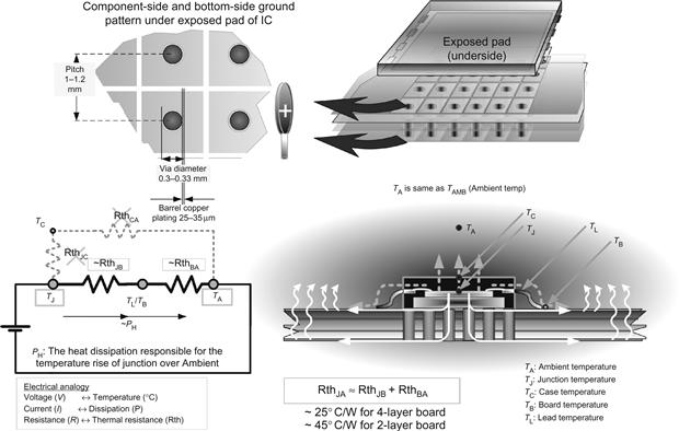
Figure 11.1: Thermal resistance explained and the correct way to mount a power IC on a board.

The figure shows the proper way of soldering down a modern device with an exposed (metal) pad on its underside, on a copper island placed on the component side of a standard four-layer board. The idea is to get the heat out quickly from the device, transfer it via thermal conduction to different parts of the PCB, including the underside (which has a similar copper island right under the exposed pad). Incidentally, FR4 (standard PCB material) is not a bad conductor of heat itself. However, a large ground plane right below the component side helps push the heat out further across the board. Finally, all the exposed PCB surfaces (including all the exposed copper on the board, not necessarily even connected to the exposed pad) behave as heatsinks. Air flows past these surfaces, taking heat away by convection. Finally, the system stabilizes at a certain temperature of interest.

In Figure 11.1, we see there is a primary path for the heat to flow via thermal conduction. This is from junction to lead/exposed pad/board through which most of the dissipation P_H goes. We can usually ignore the parallel path going from junction to case and case to ambient (because it has a very high thermal resistance). In the figure, we also see the complete electrical analog. Thermal resistance is analogous to resistance and dissipation to current. The temperature (difference) is analogous to voltage (difference).

In Figure 11.1, some recommendations on the dimensions and spacing of the “thermal vias” under the exposed pad are provided. The idea is to prevent solder wicking during the soldering reflow process, which will suck solder and possibly create a bad joint under the exposed pad, thereby compromising the entire thermal performance. Note that the thermal vias are sometimes prefilled with copper. That prevents solder wicking and improves the conduction capability of the thermal vias themselves. But it is more costly.

Finally, we note that most power devices have a relatively low Rth_JL. So, the net junction to ambient thermal resistance Rth_JA is predominantly comprised of Rth_LA. But that is basically just the thermal resistance of the PCB (to ambient) and has almost nothing to do with the package or device itself. Which is why in Figure 11.1, we have indicated that for most modern power devices on four-layer boards, with a stackup and build as indicated in Figure 11.1, we can safely assume Rth_JA≈25°C/W for estimating T_J. Similarly, for a two-layer board, since the inner ground plane is missing (all else remaining the same), the thermal resistance is about 45°C/W. We can use these numbers (or better Rth data provided by the vendor) to estimate temperature rise as shown in the last solved example of Chapter 19.

When we mount a power semiconductor (like a TO-220 or TO-247 device in AC–DC applications) on a proper heatsink (denoted by “H”) we can write similarly

The final junction temperature is therefore

So, if we know the thermal resistance of the heatsink, we can guess the junction temperature quite accurately. Empirical equations exist, based on the area of the heatsink, to estimate the effectiveness of heatsinks (plate types in particular). They can be applied to PCBs too with some qualifications as discussed next.

Historical Definitions

We take the simplest case of a square plate made from a very good thermally conducting material, dissipating P Watts. After some time, we will find that the plate stabilizes at a certain temperature rise of “ΔT” over the ambient.

We expect that the temperature rise will be proportional to the dissipation. The “proportionality constant” is called the thermal resistance “Rth” in °C/W. So,

Similarly, we expect that the thermal resistance will vary inversely with the area:

We expect to define another proportionality constant here.

Stop: What is the area we are referring to here? If we have a plate 3 in.×3 in., we say that its area is 9 sq.in. However, the area exposed to natural convection is actually twice that — 18 sq.in. (both sides). This is one major source of confusion in using and comparing the various empirical equations provided in literature — some refer to “A” as the total exposed area, and some refer to the area of one side. Therefore, to avoid confusion we have adopted the following convention here.

“A” refers to the area of one side of a plate, whose both sides are exposed to cooling. The total exposed area is “ A ” (so A=2 A).

Using our terminology, the inverse of the proportionality constant above is “h” in W/°C per unit area and is called by various names like “convection coefficient” or “heat transfer coefficient.”

Finally, we have the basic equations

Explicitly for h,

And also,

It was originally thought that “Rth” and “h” were constants, and that was the intent of writing the classical equations as presented above. Later it was realized that the equations were not very accurate for various reasons. However, the equations presented above were maintained. What changed was that “h” or “Rth” were now “allowed” to depend on area, dissipation, and so on, all the factors they were supposedly independent of. Note that the dependency is not very severe, and so even today, we often assume that Rth and h are constants to a first approximation.

Empirical Equations for Natural Convection

As a first approximation, h is often stated in literature (at sea-level) as

If area is expressed in meters, this becomes

since there are 39.37 in. in a meter.

Nowadays we know that in reality, “h” can vary about 1:4 times from the commonly assumed typical values above.

So, in literature we can find the following generalized empirical equation for h, and this becomes our standard equation no. 1:

where L is the length along the direction of natural convection (vertical). In the case of the simple square plate, L=A^0.5, so we can write this as

Observe that the above equation uses “A” which is actually half the area exposed to cooling. So, we can equivalently rewrite it in terms of the actual area involved in the cooling process:

These are all available and published forms of the same equation for h. If the different forms are not recognized as one, it is easy to get confused and not know which equation to pick.

The above equation predicts that “h” has a specified dependency on the exposed area of the plate and also on its temperature differential with respect to ambient. This dependency (i.e., A^−0.125) implies that the cooling efficiency per unit area (i.e., “h”) of large plates is worse than that of small plates. However, if this sounds surprising, we note that the overall/total cooling efficiency of a plate is h×A, which depends on A^−0.125×A=A^0.875. So, thermal resistance of a plate goes as 1/A^0.875 and is clearly lower for a large plate than for a small plate as we would expect. Compare this to the “ideal” 1/A variation which was, classically speaking, expected for thermal resistance.

In literature, we often find the following “standard” formula (area in sq. in.), hereafter referred to as our standard equation no. 2:

We notice that the first equation is written in terms of “h” and the second in terms of “Rth.” How do we compare them? We can do some manipulations on these equations to bring them to a comparable format. We can rewrite our standard equation no. 1 in terms of dissipation instead of temperature rise:

So,

Or in terms of the total exposed area:

We can also now try to see what this will look like in MKS (SI) units. The conversion is not obvious and so we proceed as follows.

Take an imaginary plate of size 39.37 in.×39.37 in. or 1 m×1 m. Clearly, the thermal resistance of the plate is in °C/W and is therefore independent of the units used to measure area, and must remain unchanged by any change in the system of units used. This means that 1/(h×A) is independent of units, and so is h×A. Therefore, if in MKS units we first assume a similar form for h:

Equating,

So, finally in MKS units

This is also a common form seen in literature, often thought to be a separate equation altogether.

Comparing the Two Standard Empirical Equations

We basically just have two equations to choose from. Our standard equation no. 2 is

The result of manipulations on standard equation no. 1 gives us

Both these use the area of one side of the plate, though it is assumed both sides are exposed to natural convection. And we thus see that the two equations, one initially expressed in terms of h and the other in terms of Rth, are not very different at all, if brought to a similar form as we have done above.

In Figure 11.2, we have compared these two commonly seen equations (with their numerous almost unrecognizable forms). We realize all the equations commonly seen in literature are actually just two equations, both of which when plotted out, as in Figure 11.2, are very close. We can pick the dotted lines (standard equation no. 2, as the more conservative).

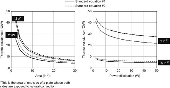
Figure 11.2: Plotting out the two standard empirical natural convection equations of plate heatsinks.

Sizing Copper Traces

There are complicated curves available for copper versus temperature rise of PCB traces in the now-obsolete standard “MIL-STD-275E.” These curves have also found their way into more recent standards like IPC-2221 and IPC-2222. Engineers often try to create elaborate curve fit equations to match these curves. But the truth is the earlier curves can be easily approximated by simple linear rules as follows.

The required cross-sectional area of an external trace is approximately

For the traces in inner layers, multiply the calculated width of an external trace by 2.6 to get the required width.

To calculate width of a trace from the cross-sectional area, keep in mind that 1-oz copper is 1.4 mils thick and 2-oz copper is 2.8 mils thick.

Natural Convection at an Altitude

At sea-level, over 70% of heat is transferred by natural convection and the rest by radiation. Only at very high altitudes (70,000 ft+), the ratio inverts and the heat lost by radiation could be 70–90% of the total, even though the radiated transfer is unchanged. So by about 10,000 ft the overall efficiency of cooling typically falls to 80%, at 20,000 it is only 60%, and at 30,000 it is 50%.

Knowing that the coefficient of natural convection goes as P^1/2, where P is the pressure of air, a good curve fit gives us the following useful relationship:

So, for example, we find that at 10,000 ft, all the Rth’s at sea-level need to be increased by about 19.5%.

Forced Air Cooling

Fans are rated for a certain cubic feet of minute “cfm.” The actual cooling, however, depends on the linear feet per minute “lfm” to which the heatsink is subjected. Two parameters are needed to find the velocity in lfm: (1) the volume of air discharged from the fan in cfm and (2) the cross-sectional area through which the cooling air passes in m². So lfm=cfm/Area. But, finally, we should derate the calculated lfm by 60–80% to account for backpressure.

At sea-level, the following formula gives a rough estimate of the required airflow:

The ΔT is the differential between the inlet and the outlet temperatures. It is typically set to about 10–15°C.

Note that if the inlet temperature, which is the room ambient, is 55°C for example, then we need to add this differential ΔT as the actual local ambient inside the power supply when doing our initial calculations. However, ultimately we will be carrying out an actual temperature test by attaching thermocouples to all the components. We will thus certainly see an advantage in moving hotter components closer to the inlet during the design phase.

The linear speed is often expressed in terms of m/s. 1 m/s is equal to an lfm of 196.85. Roughly, 1 m/s is 200 lfm.

Some empirical results are as follows: at 30-W dissipation, an unblackened plate of 10 cm×10 cm has the following Rth: 3.9°C/W under natural cooling, 3.2°C/W with 1 m/s, 2.4°C/W with 2 m/s, and 1.2°C/W with 5 m/s. Provided the air flows parallel to the fins, with speed >0.5 m/s, the thermal resistance hardly depends on the power dissipation. That is because, on its own, even in static air, hot plates produce enough air movement around them to help in the heat transfer. Also note that blackening of plates has some effect under natural convection, but curves for forced convection depend very little on this aspect. Radiation is improved by blackening, but at sea-level that is only a small part of the overall heat transfer. In general, black anodized heatsinks still seen in some forced air designs are actually a waste and should be replaced with uncoated aluminum.

Under steady-state, roughly 2 mm thick copper is almost exactly equivalent to 3 mm thick aluminum. The only advantage of copper is its better thermal conductivity, so it may be used to avoid thermal constriction effects when using very large areas.

The curve of thermal resistance to air flow falls off roughly exponentially, and so the improvement in thermal resistance in going from still air to 200 lfm is the same as from 200 lfm to 1,000 lfm. Velocities in excess of 1,000 lfm (about 5 m/s) do not cause significant improvement.

Under forced convection, the Nusselt number at sea-level is

Note that generally for natural convection, we can assume laminar flow. But under high dissipation, the hot air tends to rise so fast that it breaks up into turbulence. This is actually very useful in reducing the thermal resistance (increasing the “h”). For forced air convection, it is common to cut fingers on the sides of plate metal sinks and bend them alternately in and out. The purpose here is to actually create turbulent flow in the vicinity of the heatsink, thus lowering its thermal resistance. However, we do note from the formal analysis and equations which follow, turbulent flow provides better cooling (high “h”) under conditions of high lfm and/or large plates only. Laminar flow will provide better cooling otherwise.

Above we have defined the Prandtl number “Pr,” which is the ratio of momentum diffusion to thermal diffusion. We can take its value at sea-level to be 0.7. “Re” is the dimensionless Reynolds’s number, which is the ratio of momentum flow to viscous flow. If the plate has two dimensions L1 and L2 (so that L1×L2=A), and L1 is the dimension along the flow of air, then Re is

where we already know ν=15.9×10⁻⁶ (the kinematic viscosity in m²/s). Thus, we get the h under forced convection:

where K_AIR is the thermal conductivity of air (0.026 W/m-°C). Putting all the numbers together, we simplify to get

At higher altitudes, we need to increase the cfm calculated at sea-level by the following factor so as to maintain the same effective cooling. This is because a fan is a constant volume mover, not a constant mass mover, and at high altitudes, the air density is much lower. Therefore, the cfm has to be increased in inverse proportion to the pressure.

For example, at 10,000 ft, the calculated cfm at sea-level has to be increased by 43% to maintain the same h_FORCED.

Radiative Heat Transfer

Radiation does not depend on air, and can take place even in vacuum, since it is electromagnetic in nature. At high altitudes, radiative heat transfer can become a significant part of the overall heat transfer. The equation for “h” is

ε is the emissivity of the surface. It is 1 for a perfect blackbody, but for polished metal surfaces we should take this as 0.1. If the surface is anodized, we can take it as about 0.9.

Note that at high altitudes, under forced air cooling, the cfm falls, and so the inlet-to-outlet ΔT increases somewhat. Therefore, T_AMB goes up, and this affects h_RAD. So, it may end up looking like radiation is getting affected at higher altitudes too, but it is for a different reason altogether (rise in ambient).

Miscellaneous Issues