
9 Information extraction from medical images: evaluating a novel automatic image annotation system using semantic-based visual information retrieval
Abstract: Today, in the medical field there are huge amounts of non-textual information, such as radiographic images, generated on a daily basis. Given the substantial increase of medical data stored in digital libraries, it is becoming more and more difficult to perform search and information retrieval tasks. Image annotation remains a difficult task for two reasons: (1) the semantic gap problem –it is hard to extract semantically meaningful entities when using low-level image features; and (2) the lack of correspondence between the keywords and image regions in the training data. Content-based visual information retrieval (CBVIR) and image annotation has attracted a lot of interest, namely from the image engineering, computer vision, and database community. Unfortunately, current methods of the CBVIR systems only focus on appearance-based similarity, i.e., the appearance of the retrieved images is similar to that of a query image. As a result, there is very little semantic information exploited. To develop a semantic-based visual information retrieval (SBVIR) system two steps are required: (1) to extract the visual objects from images; and (2) to associate semantic information with each visual object. The first step can be achieved by using segmentation methods applied to images, while the second step can be achieved by using semantic annotation methods applied to the visual objects extracted from images. In this chapter, we use original graph-based color segmentation methods because we find that as linear algorithms they perform well. The annotation process implemented in our system is based on the Cross-Media Relevance Model (CMRM), which invokes principles defined for relevance models. For testing the annotation module, we have used a set of 2000 medical images: 1500 of images in the training set and 500 test images. For testing the quality of our segmentation algorithm, the experiments were conducted using a database consisting of 500 medical images of the digestive system that were captured by an endoscope. Our initial test results, based on looking at the assigned words to see if they were relevant to the image in question, have proven that our automatic image annotation system augurs well in the diagnostic and treatment process. This is first step toward larger studies of automatic image annotation for indexing, retrieving, and understanding large collections of image data.
9.1 Introduction
Advances in medical technology generate huge amounts of non-text information (e.g., images) along with more familiar textual one. Medical images play a central role in patient diagnosis, therapy, surgical planning, medical reference, and medical training. The image is one of the most important tools in medicine since it provides a method for diagnosis and monitoring of patients’ illnesses and conditions, with the advantage of it being a very fast, non-invasive procedure. Automatic image-annotation (also known as automatic image tagging or linguistic indexing) is the process by which the computer system automatically assigns metadata, in the form of captioning or keywords, to the digital image while taking into account its content. This process is of great value as it allows indexing, retrieving, and understanding of large collections of image data. As new image acquisition devices are continually developed to produce more accurate information and increase efficiency, and as data storage capacity likewise increases, a steady growth in the number of medical images produced can be easily inferred. Given the massive increase of medical data in digital libraries, it is becoming more and more difficult to perform search and information retrieval tasks. In sum, image annotation remains a difficult task for two main reasons: (1) the semantic gap problem – it is hard to extract semantically meaningful entities when using low-level image features; and (2) the lack of correspondence between the keywords and image regions in the training data.
Recently, there has been lot of discussion about semantically-enriched information systems, especially about using ontology for modeling data. In this chapter, we present a novel image-annotation system, revolving on a more comprehensive information extraction approach, for use in the medical domain. The annotation model used was inspired from the principles defined for the cross-media relevance model. The ontology used by the annotation process was created in an original manner starting from the information content provided by the medical subject headings (MeSH). Our novel approach is based on the double assumption that given images from digestive diseases, expressing all the desired features using domain knowledge is feasible; and that manually marking up and annotating the regions of interest is practical as well. In addition, by developing an automatic annotation system, representing and reasoning about medical images are performed with reasonable complexity within a given query context. Not surprisingly, due to the presence of a large number of images without text information, content-based medical image retrieval has received quite a bit of attention in recent years.
9.2 Background
Content-based visual information retrieval (CBVIR) has attracted a lot of interest, namely from the image engineering, computer vision and database community. A large corpus of research has been built up in this field showing substantial results. Content-based image retrieval task could be described as a process for efficiently retrieving images from a collection by similarity. The retrieval relies on extracting the appropriate characteristic quantities describing the desired contents of images. Most CBVIR approaches rely on the low-level visual features of image and video, such as color, texture and shape. Such techniques are called feature-based techniques in visual information retrieval (Tousch et al. 2012). Unfortunately, current methods of the CBVIR systems only focus on appearance-based similarity, i.e., the appearance of the retrieved images is similar to that of a query image. As a result, there is very little semantic information exploited. Among the few efforts which claim to exploit the semantic information, the semantic similarities are defined between different appearances of the same object. These kinds of semantic similarities represent the low-level semantic similarities, while and the similarities between different objects represent the high-level semantic similarities. The similarities between two images are the similarities between the objects contained within the two images. As a consequence, a way to develop a semantic-based visual information retrieval (SBVIR) system consists of two steps: (1) to extract the visual objects from images; and (2) to associate semantic information with each visual object. The first step can be achieved by using segmentation methods applied to images, while the second step can be achieved by using semantic annotation methods applied to the visual objects extracted from images.
Image segmentation techniques can be separated into two groups: region-based and contour-based approaches. Region-based segmentation methods can be broadly classified as either top-down (model-based) or bottom-up (visual feature-based) approaches (Adamek et al. 2005).
An important group of visual feature-based methods is represented by the graph-based segmentation methods, which attempt to search for certain structures in the associated edge-weighted graph constructed on the image pixels, such as minimum spanning tree or minimum cut. Other approaches to image segmentation which are region-based consist of splitting and merging regions according to how well each region fulfills some uniformity criterion. Such methods use a measure of uniformity of a region. In contrast, other region-based methods use a pair-wise region comparison rather than applying a uniformity criterion to each individual region. Liew & Yan (2005) demonstrate that the contour-based segmentation approach, as distinguished from region-based approach, assumes that different objects in an image can be segmented by detecting their boundaries. The authors further sharpen the distinction between these two groups: “whereas region-based techniques attempt to capitalize on homogeneity properties within regions in an image, boundary-based techniques [used in the contour-based approach] rely on the gradient features near an object boundary as a guide” (p. 316).
Medical images segmentation describes some graph-based color segmentation methods, and an area-based evaluation framework of the performance of the segmentation algorithms.
The proposed SBVIR system involves an annotation process of the visual objects extracted from images. It becomes increasingly expensive to manually annotate medical images. Consequently, automatic medical image annotation becomes important. We consider image annotation as a special classification problem, i.e., classifying a given image into one of the predefined labels.
Several interesting techniques have been proposed in the image annotation research field. Most of these techniques define a parametric or non-parametric model to capture the relationship between image features and keywords (Stumme & Maedche 2001). The concepts used for annotation of visual objects are generally structured in hierarchies of concepts that form different ontologies. The notion of ontology is defined as an explicit specification of some conceptualization, while the conceptualization is defined as a semantic structure that encodes the rules of constraining the structure of a part of reality. The goal of ontology is to define some primitives and their associated semantics in some specified context. Ontology has been established for knowledge sharing and is widely used as a means for conceptually structuring domains of interest. With the growing usage of ontology, the problem of overlapping knowledge in a common domain occurs more often and becomes critical. Domain-specific ontology is modeled by multiple authors in multiple settings. Such an ontology lays the foundation for building new domain specific ontology in similar domains by assembling and extending ontology from repositories. Though ontology is frequently used in the medical domain, existing ontology is provided in formats that are not always easy to interpret and use. To handle these uncertainties, researchers have proposed a great number of annotation models and information extraction techniques (Stanescu et al. 2011).
9.3 Related work
Because ontology are not always easy to interpret, a number of models using a discrete image vocabulary have been proposed for image annotation (Mori, Takahashi & Oka 1999; Duygulu et al. 2002; Barnard et al. 2003; Blei & Jordan 2003; Jeon, Lavrenko & Manmatha 2006; Lavrenko, Manmatha & Jeon 2006). One approach to automatically annotating images is to look at the probability of associating words with image regions. Mori, Takahashi & Oka (1999) used a co-occurrence model where they looked at the co-occurrence of words with image regions created using a regular grid. To estimate the correct probability this model required large numbers of training samples. Thus, the co-occurrence model, translation model (Duygulu et al. 2002), and the cross-media relevance model (CMRM) (Jeon, Lavrenko & Manmatha 2003) demonstrates that each is respectively trying to improve a previous model.
Annotation of medical images requires a nomenclature of specific terms retrieved from ontology to describe its content. For medical domain what can be used is either an existing ontology named open biological and biomedical ontology (http://www.obofoundry.org/) or a customized ontology based on a source of information from a specific domain.
The medical headings (MeSH) (http://www.nlm.nih.gov/) and (http://en.wikipedia.org/wiki/Medical_Subject_Headings) are produced by the National Library of Medicine (NLM) and contain a high number of subject headings, also known as descriptors. MeSH thesaurus is a vocabulary used for subject indexing and searching of journal articles in MEDLINE/PubMed (http://www.ncbi.nlm. nih.gov/pubmed). MeSH has a hierarchical structure (http://www.nlm.nih.gov/mesh/2010/mesh_browser/MeSHtree.html) and contains several top level categories like anatomy, diseases, health care, etc. Relationships among concepts (http://www.nlm.nih.gov/mesh/meshrels.html) can be represented explicitly in the thesaurus as relationships within the descriptor class. Hierarchical relationships are seen as parent-child relationships and associative relationships are represented by the “see related” cross reference.
Duygulu et al. (2002) described images using a vocabulary of blobs (which are clusters of image regions obtained using the K-means algorithm). Image regions were obtained using the normalized-cuts segmentation algorithm. For each image region 33 features such as color, texture, position and shape information were computed. The regions were clustered using the K-means clustering algorithm into 500 clusters called “blobs.” This annotation model called translation model was a substantial improvement of the co-occurrence model. It used the classical IBM statistical machine translation model (Brown et al. 1993) making a translation from the set of blobs associated to an image to the set of keywords for that image.
Jeon et al. (2003) viewed the annotation process as analogous to the cross-lingual retrieval problem and used a cross media relevance model to perform both image annotation and ranked retrieval. The experimental results have shown that the performance of this model on the same dataset was considerably better than the models proposed by Duygulu et al. (2002) and Mori et al. (1999).
There are other models like correlation LDA proposed by Blei & Jordan (2003) that extends the Latent Dirichlet Allocation model to words and images. This model is estimated using expectation-maximization algorithm and assumes that a Dirichlet distribution can be used to generate a mixture of latent factors. In Li & Wang (2003) it is described a real-time ALIPR image search engine which uses multi resolution 2D hidden Markov models to model concepts determined by a training set. In an alternative approach, Blei & Jordan (2003) rely on a hierarchical mixture representation of keyword classes, leading to a method that has a computational efficiency on complex annotation tasks. There are other annotation systems used in the medical domain like I2Cnet (Image indexing by Content network) Catherine, Xenophon & Stelios (1997) providing services for the content-based management of images in health care. In Igor et al. (2010), the authors present a hierarchical medical image annotation system using Support Vector Machines (SVM) – based approaches.
In Daniel (2003) the author provides an in depth description of Oxalis, a distributed image annotation architecture allowing the annotation of an image with diagnoses and pathologies. In Baoli, Ernest & Ashwin (2007) the authors describe the SENTIENT-MD (Semantic Annotation and Inference for Medical Knowledge Discovery) a new generation medical knowledge annotation and acquisition system.
In Peng, Long & Myers (2009) the authors present VANO, a cross-platform image annotation system enabling the visualization and the annotation of 3D volume objects including nuclei and cells.
Some of the elements (e.g., the clustering algorithm used for obtaining blobs or the probability distribution of the CMRM) included in our system are related to Soft Computing which is an emerging field that consists of complementary elements of fuzzy logic, neural computing, evolutionary computation, machine learning and probabilistic reasoning. Machine learning includes unsupervised learning which models a set of inputs, like clustering.
9.4 Architecture of system
The annotation process implemented in our system is based on the cross-media relevance model (CMRM), which invokes principles defined for relevance models. Using a set of color-annotated images of the diseases of the digestive system, the system learns the distribution of the blobs and words. The diseases are indicated in images by color and texture changes. Having the set of blobs, each image from the test set is then represented using a discrete sequence of blobs identifiers. The distribution is used to generate a set of words for a new image.
The architecture of our system is presented in Fig. 9.1 and contains six modules (Burdescu et al. 2013):
- – Segmentation module – these modules segment an image into regions by planar segmentation; it can be configured to segment all images from an existing images folder on the storage disk. The hexagonal structure used by the owner segmentation algorithm represents a grid-graph and is presented in Fig. 9.2. For each hexagon “h” in this structure there exist 6-hexagons that are neighbors in a 6-connected sense. The segmentation process is using some methods in order to obtain the list of regions:
- – Same vertex color – used to determine the color of a hexagon
- – Expand colour area – used to determine the list of hexagons having the color of the hexagon used as a starting point and has as running time where n is the number of hexagons from a region with the same color.
- – List regions – used to obtain the list of regions and has as running time where n is the number of hexagons from the hexagonal network.
- – Characteristics extractor module – this module is using the regions detected by the Segmentation module. For each segmented region is computed a feature vector that contains visual information of the region such as color (color histogram with 166 bins, texture (maximum probability, inverse difference moment, entropy, energy, contrast, correlation), position (minimum bounding rectangle) and shape (area, perimeter, convexity, compactness). The components of each feature vector are stored in the database.
- – Clustering module – we used K-means with a fixed value of 80 (established during multiple tests) to quantize these feature vectors obtained from the training set and to generate blobs. After the quantization, each image in the training set is represented as a set of blobs identifiers. For each blob it is computed a median feature vector and a list of words belonging to the test images that have that blob in their representation.
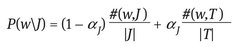
- – Annotation module – for each region belonging to a new image it is assigned the blob which is closest to it in the cluster space. The assigned blob has the minimum value of the Euclidian distance computed between the median feature vector of that blob and the feature vector of the region. In this way the new image will be represented by a set of blobs identifiers. Having the set of blobs and for each blob having a list of words we can determine a list of potential words that can be assigned to the image. What needs to be established is which words describe better the image content. This can be made using the formulas of the cross media relevance model:
(1)
where: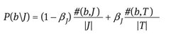
(2)
- – P(w|J) , P(b|J) denote the probabilities of selecting the word “w,” the blob “b” from the model of the image J.
- – #(w,J) denotes the actual number of times the word “w” occurs in the caption of image J.
- – #(w,T) is the total number of times “w” occurs in all captions in the training set T.
- – #(b,J) reflects the actual number of times some region of the image J is labeled with blob “b.”
- – #(b,T) is the cumulative number of occurrences of blob “b” in the training set.
- – |J| stands for the count of all words and blobs occurring in image J.
- – |T| denotes the total size of the training set.
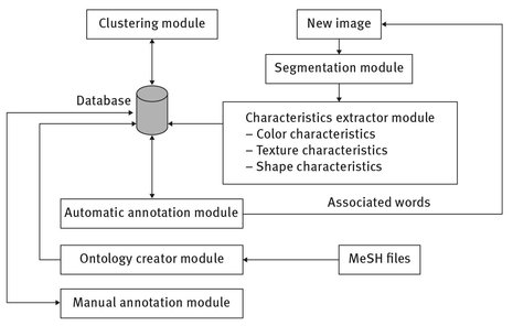
Fig. 9.1: System’s architecture.
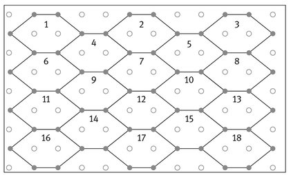
Fig. 9.2: Hexagonal structure constructed on the image pixels.
The smoothing parameters alpha and beta determine the degree of interpolation between the maximum likelihood estimates and the background probabilities for the words and the blobs, respectively. The values determined after experiments for the cross media relevance model were alpha = 0.1 and beta = 0.9. For each word is computed the probability to be assigned to the image an after that the set of “n” (configurable value) words having a high probability value will be used to annotate the image. We have used five words for each image.
Ontology creator module – this module has as input the MeSH content that can be obtained from (http://www.nlm.nih.gov/mesh/filelist.html) and is offered as an “xml” file named desc2010.xml (2010 version) containing the descriptors and a “txt” file named mtrees2010.txt containing the hierarchical structure.
This module generates the ontology and stores it in the database. This module also offers the possibility to export the ontology content as a Topic Map ( http://www.topicmaps.org/) by generating an *.xtm file using the “xtm” syntax.
The ontology contains:
- – Concepts – each descriptor is mapped to an ontology concept having as unique identifier the content of the DescriptorUI xml node. The name of the concept is retrieved from the DescriptorName xml node. The tree node of this concept in the hierarchical structure of the ontology is established using the tree identifiers existing in the TreeNumber xml nodes. Usually a MeSH descriptor can appear in multiple trees. For the descriptor mentioned in the above example the concept will have the following properties
- – id:D000001, name:Calcimycin, tree_nodes: D03.438.221.173
- – Associations defined between concepts – our ontology contains two types of associations:
- – parent-child – generated using the hierarchical structure of the MeSH trees and the tree identifiers defined for each concept (used to identify the concepts implied in the association)
- – related-to – a descriptor can be related to other descriptors. This information is mentioned in the descriptor content by a list of DescriptorUI values. In practice a disease can be caused by other diseases.
- – Manual annotation module – this module is used to obtain a training set of annotated images needed for the automatic annotation process. This module is usually used after the following steps are completed:
- – the doctor obtains a set of images collected from patients using an endoscope and this set is placed in a specific disk location that can be accessed by our segmentation module
- – the segmentation module segments each image from the training set
- – the set of regions obtained after segmentation is processed by the characteristics’ extractor module and all characteristic vectors are stored in the database
- – the clustering module using the k-means algorithm generates the set of blobs and each image is represented by a discrete set of blobs.
The manual annotation module has a graphical interface, which allows the doctor to select images from the training set to see the regions obtained after segmentation and to assign keywords from the ontology created for the selected image.
9.5 The segmentation algorithm – graph-based object detection (GBOD)
Segmentation is the process of partitioning an image into non-intersecting regions such that each region is homogeneous and the union of no two adjacent regions is homogeneous. Formally, segmentation can be defined as follows.
Let F be the set of all pixels/voxels and P() be a uniformity (homogeneity) predicate defined on groups of connected pixels/voxels, then segmentation is a partitioning of the set F into a set of connected subsets or regions (S1, S2, . . ., Sn) such that ∪ni =1Si = F with Si ∩ Sj = Ø when i ≠ j. The uniformity predicate P(Si) is true for all regions Si and P(Si ∪ Sj) is false when Si is adjacent to Sj.
This definition can be applied to all types of images.
The goal of segmentation is typically to locate certain objects of interest which may be depicted in the image. Segmentation could therefore be seen as a computer vision problem. A simple example of segmentation is to threshold a grayscale image with a fixed threshold “t”: each pixel/voxel “p” is assigned to one of two classes, P0 or P1, depending on whether I(p) < t or I(p) > = t.
Grouping can be formulated as a graph partitioning and optimization problem by Pushmeet Kohli et al. (2012) and C. Allène et al. (2010).
The graph theoretic formulation of image segmentation is as follows:
- The set of points in an arbitrary feature space are represented as a weighted undirected graph G = (V,E), where the nodes of the graph are the points in the feature space
- An edge is formed between every pair of nodes yielding a dense or complete graph.
- The weight on each edge, w(i,j) is a function of the similarity between nodes i and j.
- Partition the set of vertices into disjoint sets V1, V2, . . ., Vk where by some measure the similarity among the vertices in a set Vi is high and, across different sets Vi, Vj is low.
To partition the graph in a meaningful manner, we also need to:
- – Pick an appropriate criterion (which can be computed from the graph) to optimize, so that it produces a clear segmentation.
- – Finding an efficient way to achieve the optimization.
In the image segmentation and data clustering community, there has been a substantial amount of previous work using variations of the minimal spanning tree or limited neighborhood set approaches (Grundmann et al. 2010). Although such approaches use efficient computational methods, the segmentation criteria used in most of them are narrowly based on local properties of the graph. However, because perceptual grouping is about extracting the global impressions of a scene, this partitioning criterion often falls short of this main goal.
There are huge of papers for 2D images and segmentation methods and most graph-based for 2D images and few papers for spatial segmentation methods. Because we used an original segmentation algorithm, we depict only the set of hexagons constructed on the image Burdescu et al. (2009); Brezovan et al. (2010); and Stanescu et al. (2011).
The method we use pivots on a general-purpose segmentation algorithm, which produces good results from two different perspectives: (1) from the perspective of perceptual grouping of regions from the natural images (standard RGB); and (2) from the perspective of determining regions if the input images contain salient visual objects.
Let V = {h1, …, h|v|} be the set of hexagons/tree-hexagons constructed on the spatial image pixels/voxels as presented above and G = (V,E) be the undirected spatial grid-graph, with E containing pairs of honey-beans cell (hexagons for planar and tree-hexagons for spatial) that are neighbors in a 6/20-connected sense. The weight of each edge e = (hi,hj) is denoted by w(e), or similarly by w(hi,hj), and it represents the dissimilarity between neighboring elements “hi” and “hj” in a some feature space. Components of an image represent compact regions containing pixels/voxels with similar properties. Thus, the set V of vertices of the graph G is partitioned into disjoint sets, each subset representing a distinct visual object of the initial image.
As in other graph-based approaches Burdescu et al. (2009) we use the notion of segmentation of the set V. A segmentation, S, of V is a partition of V, such that each component C ∈ S corresponds to a connected component in a spanning sub-graph GS = (V,ES) of G, with ES ⊆ E.
The set of edges E−ES that are eliminated connect vertices from distinct components. The common boundary between two connected components C′,C′′ ∈ S represents the set of edges connecting vertices from the two components:
(3)
The set of edges E−ES represents the boundary between all components in S. This set is denoted by bound(S) and it is defined as follows:
(4)
In order to simplify notations throughout the paper we use Ci to denote the component of a segmentation S that contains the vertex hi ∈ V.
We use the notions of segmentation “too fine” and “too coarse” as defined in Felzenszwalb & Huttenlocher (2004) that attempt to formalize the human perception of salient visual objects from an image. A segmentation S is too fine if there is some pair of components C′,C′′ ∈ S for which there is no evidence for a boundary between them. S is too coarse when there exist a proper refinement of S that is not too fine. The key element in this definition is the evidence for a boundary between two components.
The goal of a segmentation method is to determine a proper segmentation, which represent visual objects from an image.
Definition 1 Let G = (V,E) be the undirected planar/spatial graph constructed on the hexagonal/tree-hexagonal structure of an image, with V = {h1, …, h|V|}. A proper segmentation of V, is a partition S of V such that there exists a sequence [Si, Si+1, …, Sf−1, Sf ] of segmentations of V for which:
- – S = Sf is the final segmentation and Si is the initial segmentation,
- – Sj is a proper refinement of Sj+1 (i.e., Sj ⊂ Sj+1) for each j = i, …, f−1,
- – segmentation Sj is too fine, for each j = i, …, f−1,
- – any segmentation Sl such that Sf ⊂ Sl, is too coarse,
- – segmentation Sf is neither too coarse nor too fine.
We present a unified framework for image segmentation and contour extraction that uses a virtual hexagonal structure defined on the set of the image pixels. This proposed graph-based segmentation method is divided into two different steps: (1) a pre-segmentation step that produces a maximum spanning tree of the connected components of the triangular grid graph constructed on the hexagonal structure of the input image; and (2) the final segmentation step that produces a minimum spanning tree of the connected components, representing the visual objects by using dynamic weights based on the geometric features of the regions (Stanescu et al. 2011).
Each hexagon from the hexagonal grid contains eight pixels: six pixels from the frontier and two interior pixels. Because square pixels from an image have integer values as coordinates we always select the left pixel from the two interior pixels to represent with approximation the gravity center of the hexagon, denoted by the pseudo-gravity center. We use a simple scheme of addressing for the hexagons of the hexagonal grid that encodes the spatial location of the pseudo-gravity centers of the hexagons as presented in Fig. 9.3 (for planar image).
Let w × h the dimension of the initial image. Given the coordinates <h, c> of a pixel “p” from the input image, we use the linear function, ipw,h(<l, c >)= (l − 1)w + c, in order to determine an unique index for the pixel.
Let “ps” be the sub-sequence of the pixels from the sequence of the pixels of the initial image that correspond to the pseudo-gravity center of hexagons, and “hs” the sequence of hexagons constructed over the pixels of the initial image. For each pixel “p” from the sequence “ps” having the coordinates < h, c > , the index of the corresponding hexagon from the sequence “hs” is given automatically by system. Equation for the hexagons is linear and it has a natural order induced by the sub-sequence of pixels representing the pseudo-gravity center of hexagons. Relations allow us to uniquely determine the coordinates of the pixel representing the pseudo-gravity center of a hexagon specified by its index (its address). Each hexagon represents an elementary item and the entire virtual hexagonal structure represents a triangular grid graph, G = (V,E), where each hexagon “h” in this structure has a corresponding vertex v ∈ V. The set E of edges is constructed by connecting hexagons that are neighbors in a 6-connected sense. The vertices of this graph correspond to the pseudo-gravity centers of the hexagons from the hexagonal grid and the edges are straight lines connecting the pseudo-gravity centers of the neighboring hexagons, as presented in Fig. 9.3.
There are two main advantages when using hexagons instead of pixels as elementary pieces of information:
- The amount of memory space associated with the graph vertices is reduced. Denoting by “np” the number of pixels of the initial image, the number of the resulted hexagons is always less than np/4, and thus the cardinal of both sets V and E is significantly reduced;
- The algorithms for determining the visual objects and their contours are much faster and simpler in this case. Many of these algorithms are “borrowed” from graph sets Cormen et al. (1990).
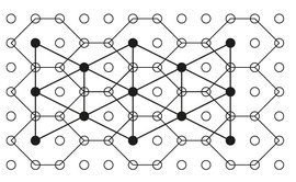
Fig. 9.3: The triangular grid graph constructed on the pseudo-gravity centers of the hexagonal grid.
We associate to each hexagon “h” from V two important attributes representing its dominant color and the coordinates of its pseudo-gravity center, denoted by “g(h).” The dominant color of a hexagon is denoted by “c(h)” and it represents the color of the pixel of the hexagon which has the minimum sum of color distance to the other seven pixels. Each hexagon “h” in the hexagonal grid is thus represented by a single point, g(h), having the color c(h). By using the values g(h) and c(h) for each hexagon information related to all pixels from the initial image is taken into consideration by the segmentation algorithm.
Our segmentation algorithm starts with the most refined segmentation, S0 = {{h1}, …, {h|V|}} and it constructs a sequence of segmentations until a proper segmentation is achieved. Each segmentation Sj is obtained from the segmentation Sj−1 by merging two or more connected components for there is no evidence for a boundary between them. For each component of a segmentation a spanning tree is constructed; thus for each segmentation we use an associated spanning forest.
The evidence for a boundary between two components is determined taking into consideration some features in some model of the image. When starting, for a certain number of segmentations the only considered feature is the color of the regions associated to the components and in this case we use a color-based region model. When the components became complex and contain too much hexagons/tree-hexagons, the color model is not sufficient and hence geometric features together with color information are considered. In this case we use a syntactic based (with a color-based region) model for regions. In addition, syntactic features bring supplementary information for merging similar regions in order to determine salient objects. Despite of the majority of the segmentation methods our method do not require any parameter to be chosen or tuned in order to produce a better segmentation and thus our method is totally adaptive. The entire approach is fully unsupervised and does not need a priori information about the image scene (Burdescu et al. 2011; Brezovan et al. 2010).
For the sake of simplicity, we will denote this region model as a syntactic-based region model.
As a consequence, we split the sequence of all segmentations,
(5),
in two different subsequences, each subsequence having a different region model,
(6),
where Si represents the color-based segmentation sequence, and Sf represents the syntactic-based segmentation sequence.
The final segmentation St in the color-based model is also the initial segmentation in the syntactic-based region model.
For each sequence of segmentations we develop a different algorithm (Stanescu et al. 2011). Moreover, we use a different type of spanning tree in each case: a maximum spanning tree in the case of the color-based segmentation, and a minimum spanning tree in the case of the syntactic-based segmentation (Cormen, Leiserson & Rivest 1990). More precisely our method determines two sequences of forests of spanning trees,
each sequence of forests being associated with a sequence of segmentations.
The first forest from Fi contains only the vertices of the initial graph, F0 = (V,Ø), and at each step some edges from E are added to the forest Fl = (V,El) to obtain the next forest, Fl+1 = (V,El+1). The forests from Fi contain maximum spanning trees and they are determined by using a modified version of Kruskal’s algorithm (Cormen, Leiserson & Rivest 1990), where at each step the heaviest edge (u,v) that leaves the tree associated to “u” is added to the set of edges of the current forest.
The second subsequence of forests that correspond to the subsequence of segmentations Sf contains forests of minimum spanning trees and they are determined by using a modified form of Boruvka’s algorithm. This sequence uses as input a new graph, G′ = (V′, E′), which is extracted from the last forest, Ft, of the sequence ![]() Each vertex “v” from the set V′ corresponds to a component Cv from the segmentation St (i.e., to a region determined by the previous algorithm). At each step the set of new edges added to the current forest are determined by each tree T contained in the forest that locates the lightest edge leaving T. The first forest from Ff contains only the vertices of the graph G′, Ft′ = (V′,Ø).
Each vertex “v” from the set V′ corresponds to a component Cv from the segmentation St (i.e., to a region determined by the previous algorithm). At each step the set of new edges added to the current forest are determined by each tree T contained in the forest that locates the lightest edge leaving T. The first forest from Ff contains only the vertices of the graph G′, Ft′ = (V′,Ø).
In this section we focus on the definition of a logical predicate that allow us to determine if two neighboring regions represented by two components, Cl′ and Cl′′, from a segmentation Sl can be merged into a single component Cl+1 of the segmentation Sl+1. Two components, Cl′ and Cl′′, represent neighboring (adjacent) regions if they have a common boundary:
(8)
We use a different predicate for each region model, color based and syntactic-based, respectively.
where the weights for the different color channels, wR, wG, and wB verify the condition
wR + wG + wB = 1.
Based on the theoretical and experimental results on spectral and real world data sets, Stanescu et al. (2011) is concluded that the PED distance with weight-coefficients (wR = 0.26, wG = 0.70, wB = 0.04) correlates significantly higher than all other distance measures including the angular error and Euclidean distance.
In the color model regions are modeled by a vector in the RGB color space. This vector is the mean color value of the dominant color of hexagons/tree-hexagons belonging to the regions. There are many existing systems for arranging and describing colors, such as RGB, YUV, HSV, LUV, CIELAV, Munsell system, etc. (Billmeyer & Salzman 1981). We have decided to use the RGB color space because it is efficient and no conversion is required. Although it also suffers from the nonuniformity problem where the same distance between two color points within the color space may be perceptually quite different in different parts of the space, within a certain color threshold it is still definable in terms of color consistency.
The evidence for a boundary between two regions is based on the difference between the internal contrast of the regions and the external contrast between them (Felzenszwalb & Huttenlocher 2004; Stanescu 2011). Both notions of internal contrast and external contrast between two regions are based on the dissimilarity between two such colors.
Let hi and hj representing two vertices in the graph G =(V,E), and let wcol(hi,hj) representing the color dissimilarity between neighboring elements hi and hj, determined as follows:
(10)
where PED(e,u) represents the perceptual Euclidean distance with weight-coefficients between colors “e” and “u,” as defined by Equation (9), and c(h) represents the mean color vector associated with the hexagons or tree-hexagon “h.” In the color-based segmentation, the weight of an edge (hi,hj) represents the color dissimilarity, w(hi,hj) = wcol(hi,hj).
Let Sl be a segmentation of the set V.
We define the internal contrast or internal variation of a component C ∈ Sl to be the maximum weight of the edges connecting vertices from C:
(11)
The internal contrast of a component C containing only one hexagon is zero: IntVar(C) = 0, if |C| = 1.
The external contrast or external variation between two components, C′,C′′ ∈ S is the maximum weight of the edges connecting the two components:
(12)
We had chosen the definition of the external contrast between two components to be the maximum weight edge connecting the two components, and not to be the minimum weight, as in Felzenszwalb & Huttenlocher W (2004) because: (1) it is closer to the human perception (perception of maximum color dissimilarity); and (2) the contrast is uniformly defined (as maximum color dissimilarity) in the two cases of internal and external contrast.
The maximum internal contrast between two components, C′,C′′ ∈ S is defined as follows:
(13)
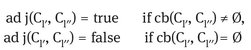
The comparison predicate between two neighboring components C′ and C′′ (i.e., adj(C′,C′′) = true) determines if there is an evidence for a boundary between C′ and C′′ and it is defined as follows:
(14)
with the the adaptive threshold ![]() (C′,C′′) given by
(C′,C′′) given by
(15)
where |C| denotes the size of the component C (i.e., the number of the hexagons or tree-hexagons contained in C) and the threshold “τ” is a global adaptive value defined by using a statistical model.
The predicate di f fcol can be used to define the notion of segmentation too fine and too coarse in the color-based region model.
Definition 2 Let G = (V,E) be the undirected spatial graph constructed on the hexagons or tree-hexagonal structure of planar or spatial image and S by color-based segmentation of V. The segmentation S is too fine in the color-based region model if there is a pair of components C′,C′′ ∈ S for which
ad j(C′,C”) = true ^ di f fcol(C′,C”) = false.
Definition 3 Let G = (V,E) be the undirected planar or spatial graph constructed on the hexagons or tree-hexagonal structure of planar or spatial image and S a segmentation of V. The segmentation S is too coarse if there exists a proper refinement of S that is not too fine.
We use the perceptual Euclidean distance with weight-coefficients (PED) as the distance between two colors.
Let G = (V,E) be the initial graph constructed on the tree-hexagonal structure of a spatial image. The proposed segmentation algorithm will produce a proper segmentation of V according to the Definition 1. The sequence of segmentations, Sif, as defined by Equation (5), and its associated sequence of forests of spanning trees, Fif, as defined by Equation (7), will be iteratively generated as follows:
- – The color-based sequence of segmentations, Si, as defined by Equation (6), and its associated sequence of forests, Fi, as defined by Equation (7), will be generated by using the color-based region model and a maximum spanning tree construction method based on a modified form of the Kruskal’s algorithm (Cormen, Leiserson & Rivest 1990).
- – The syntactic-based sequence of segmentations, Sf, as defined by Equation (6), and its associated sequence of forests, Ff, as defined by Equation (7), will be generated by using the syntactic-based model and a minimum spanning tree construction method based on a modified form of the Boruvka’s algorithm.
The general form of the segmentation procedure is presented in Algorithm 1.
Algorithm 1 Segmentation algorithm for planar images
- ** Procedure SEGMENTATION (l, c, P, H, Comp)
- Input l, c, P
- Output H, Comp
- H ←*CREATEHEXAGONALSTRUCTURE (l, c, P)
- G←*CREATEINITIALGRAPH (l, c, P, H)
- *CREATECOLORPARTITION (G, H, Bound)
- G′ ←*EXTRACTGRAPH (G,Bound,
 )
) - *CREATESYNTACTICPARTITION (G,G′,
 )
) - Comp ←*EXTRACTFINALCOMPONENTS (G′)
- End procedure
The input parameters represent the image resulted after the pre-processing operation: the array P of the planar image pixels structured in “l” lines and “c” columns. The output parameters of the segmentation procedure will be used by the contour extraction procedure: the hexagonal grid stored in the array of hexagons H, and the array Comp representing the set of determined components associated to the objects in the input image.
The global parameter threshold “![]() ” is determined by using Algorithm 1.
” is determined by using Algorithm 1.
The color-based segmentation and the syntactic-based segmentation are determined by the procedures CREATECOLORPARTITION and CREATESYNTACTICPARTITION, respectively.
The color-based and syntactic-based segmentation algorithms use the hexagonal structure H created by the function CREATEHEXAGONALSTRUCTURE over the pixels of the initial image, and the initial triangular grid graph G created by the function CREATEINITIALGRAPH. Because the syntactic-based segmentation algorithm uses a graph contraction procedure, CREATESYNTACTICPARTITION uses a different graph, G, extracted by the procedure EXTRACTGRAPH after the color-based segmentation finishes.
Both algorithms for determining the color-based and syntactic based segmentation use and modify a global variable (denoted by CC) with two important roles:
- to store relevant information concerning the growing forest of spanning trees during the segmentation (maximum spanning trees in the case of the color-based segmentation, and minimum spanning trees in the case of syntactic based segmentation),
- to store relevant information associated to components in a segmentation in order to extract the final components because each tree in the forest represents, in fact, a component in each segmentation S in the segmentation sequence determined by the algorithm.
In addition, this variable is used to maintain a fast disjoint set-structure in order to reduce the running time of the color based segmentation algorithm. The variable CC is an array having the same dimension as the array of hexagons H, which contains as elements objects of the class Tree with the following associated fields:
(isRoot, parent, compIndex, frontier, surface, color )
The field “isRoot” is a boolean value specifying if the corresponding hexagon index is the root of a tree representing a component, and the field parent represents the index of the hexagon which is the parent of the current hexagon. The rest of fields are used only if the field “isRoot” is true. The field “compIndex” is the index of the associated component.
The field “surface” is a list of indices of the hexagons belonging to the associated component, while the field “frontier” is a list of indices of the hexagons belonging to the frontier of the associated component. The field color is the mean color of the hexagon colors of the associated component.
The procedure EXTRACTFINALCOMPONENTS determines for each determined component C of Comp, the set “sa(C)” of hexagons belonging to the component, the set sp(C) of hexagons belonging to the frontier, and the dominant color c(C) of the component.
A potential user of an algorithm’s output needs to know what types of incorrect /invalid results to expect, as some types of results might be acceptable while others are not. This called for the use of metrics that are necessary for potential consumers to make intelligent decisions.
This presents the characteristics of the error metrics defined in Martin et al. (2001). The authors proposed two metrics that can be used to evaluate the consistency of a pair of segmentations, where segmentation is simply a division of the pixels of an image into discrete sets. Thus a segmentation error measure takes two segmentations S1 and S2 as input and produces a real valued output in the range [0–1] where zero signifies no error.
The process defines a measure of error at each pixel that is tolerant of refinement as the basis of both measures. A given pixel “pi” is defined in relation to the segments in S1 and S2 that contain that pixel. As the segments are sets of pixels and one segment is a proper subset of the other, then the pixel lies in an area of refinement and therefore the local error should be zero. If there is no subset relationship, then the two regions overlap in an inconsistent manner. In such case, the local error should be non-zero.
Letdenote set difference, and |x| the cardinality of set “x.” If R(S; pi) is the set of pixels corresponding to the region in segmentation S that contains pixel pi, the local refinement error is defined as in Stanescu et al. (2011):
Note that this local error measure is not symmetric. It encodes a measure of refinement in one direction only: E(S1; S2; pi) is zero precisely when S1 is a refinement of S2 at pixel “pi,” but not vice versa. Given this local refinement error in each direction at each pixel, there are two natural ways to combine the values into an error measure for the entire image. Global consistency error (GCE) forces all local refinements to be in the same direction. Let “n” be the number of pixels:
Local consistency error (LCE) allows refinement in different directions in different parts of the image.
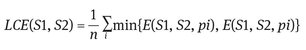
As LCE ≤ GCE for any two segmentations, it is clear that GCE is a tougher measure than LCE. Martin et al. showed that, as expected, when pairs of human segmentations of the same image are compared, both the GCE and the LCE are low; conversely, when random pairs of human segmentations are compared, the resulting GCE and LCE are high.
9.6 Experimental results
Tables 9.1 and 9.2 show the images for which we and our colleagues provide experimental results (Mihai et al. 2011).
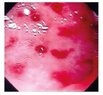
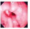
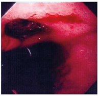
Tab. 9.1: Test Images and associated words.
| Image | Diagnostic | Words |
|---|---|---|
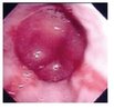 |
Esophagitis | Inflammation, esophagus, esophageal diseases, gastrointestinal diseases, digestive system diseases |
 |
Rectocolitis | Inflammation, rectum, colitis, gastroenteritis, gastrointestinal diseases |
 |
Ulcer | Peptic ulcer, duodenal diseases, intestinal diseases, gastrointestinal diseases, digestive system diseases |
For testing the annotation module, we have used a set of 2000 medical images: 1500 of images in the training set and 500 test images. In the table, below, we present the words assigned by the annotation system to some test images:
For testing the quality of our segmentation algorithm (by comparing GBOD with two other well-known algorithms – the local variation algorithm and the color-set back projection algorithm) the experiments were conducted using a database with 500 medical images of the digestive system, which were captured by an endoscope. The images were taken from patients having diagnoses such as polyps, ulcers, esophagitis, colitis, and ulcerous tumors.
Tab. 9.2: Images used in segmentation experiments.
| Image number | |
|---|---|
| 1 | 2 |
 |
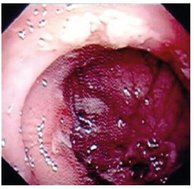 |
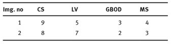
For each image the following steps are performed by the application that we have created to calculate de GCE and LCE values:
- Obtain the image regions using the color set back-projection segmentation – CS
- Obtain the image regions using the local variation algorithm (LV)
- Obtain the image regions using the graph-based object detection – GBOD
- Obtain the manually segmented regions – MS
- Store these regions in the database
- Calculate GCE and LCE
- Store these values in the database for later statistics
In Tab. 9.3 can be seen the number of regions resulted from the application of the segmentation.
Tab. 9.3: The number of regions detected for each algorithm.
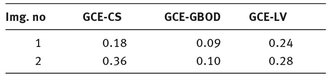
In Tab. 9.4 are presented the GCE values calculated for each algorithm.
Tab. 9.4: GCE values calculated for each algorithm.
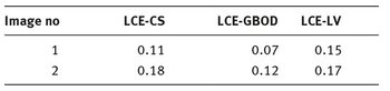
In Tab. 9.5 are presented the LCE values calculated for each algorithm.
Tab. 9.5: LCE values calculated for each algorithm.
Figures 9.4 and 9.5 present the regions resulted from manual segmentation and from the application of the segmentation algorithm presented above for images displayed in Tab. 9.2.
If a different segmentation algorithm arises from different perceptual organizations of the scene, then it is fair to declare the segmentations inconsistent. If, however, the segmentation algorithm is simply a refinement of the other, then the error should be small, or even zero. The error measures presented in the above tables are calculated in relation with the manual segmentation which is considered true segmentation. From Tabs. 9.3 and 9.4 it can be observed that the values for GCE and LCE are lower in the case of GBOD method. The error measures, for almost all tested images, have smaller values in the case of the original segmentation method, which employs a hexagonal structure defined based on the set of pixels.
Figure 9.6 presents the repartition of the 500 images from the database repartition on GCE values. The focal point here is the number of images on which the GCE value is under 0.5. In conclusion for GBOD algorithm, a number of 391 images (78%) obtained GCE values under 0.5. Similarly, for CS algorithm only 286 images (57%) obtained GCE values under 0.5. The segmentation based on LV method is close to our original algorithm: 382 images (76%) had GCE values under 0.5.
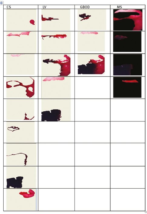
Fig. 9.4: The resulted regions for image number 1.
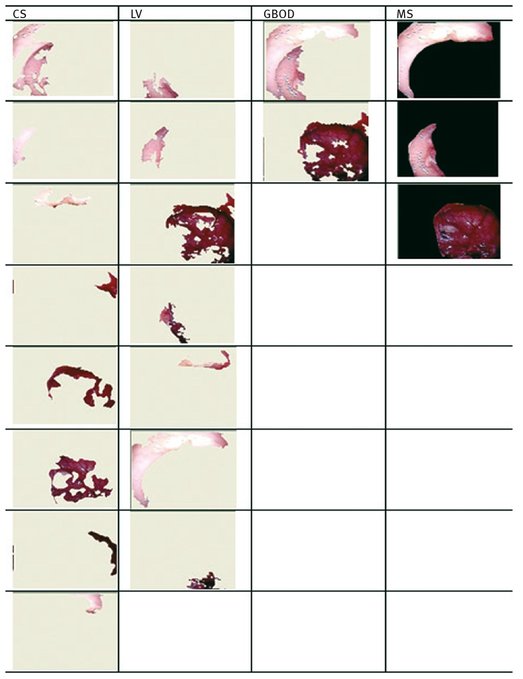
Fig. 9.5: The resulted regions for image number 2.
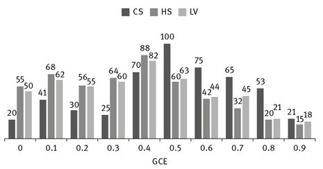
Fig. 9.6: Number of images relative to GCE values.
9.7 Conclusions
The testing scenario used by a medical doctor included the following steps: (1) A new image was obtained using the endoscope (planar and RGB image). (2) The image obtained was then processed by the annotation system and a set of words were suggested. (3) The doctor proceeded to analyze the words that were suggested along with the processed image. (4) The doctor concluded the assigned words were relevant to the image, and the system was as a starting point for the diagnostic process. Nevertheless, in order to establish and to validate a correct diagnosis of the patient’s condition, additional medical investigation is needed, inter alia, medical tests and procedures as well as a comprehensive medical history. However, by having a large enough annotated dataset of images the system can correctly suggest the diagnosis, which was the main purpose of implementing our annotation system.
In this chapter, we evaluated three algorithms used to detect regions in endoscopic images: a clustering method (the color set back-projection algorithm), as well as two other methods of segmentation based on graphs: (1) the local variation algorithm; and (2) our original segmentation algorithm (GBOD). Our method is based on a hexagonal structure defined on the set of image pixels. The advantage of using a virtual hexagonal network superimposed over the initial image pixels is that it reduces the execution time and the memory space used, without losing the initial resolution of the image.
Furthermore, because the error measures for segmentation using GBOD method are lower than for color set back-projection and local variation segmentation, we can infer that the proposed segmentation method based on a hexagonal structure is more efficient. Our experimental results show that the original GBOD segmentation method is a good refinement of the manual segmentation.
In comparison to other segmentation methods, our algorithm is able to adapt and does not require either parameters for establishing the optimal values or sets of training images to set parameters. More specifically, following our application of the three algorithms used to detect regions in radiographic images, we saw direct evidence of the adaptation of our methods when we compared the correctness of the image segments to the assigned words. Our study findings conclusively showed that concerning the endoscopic database, all the algorithms have the ability to produce segmentations that comply with the manual segmentation made by a medical expert. As part of our experiment, we used a set of segmentation error measures to evaluate the accuracy of our annotation model.
Medical images can be described properly only by using a set of specific words. In practice, this constraint can be satisfied by the usage of ontology. Several design criteria and development tools were presented to illustrate the means available for creating and maintaining ontology. All in all, building ontology for representing medical terminology systems is a difficult task that requires a profound analysis of the structure and the concepts of medical terms, but necessary in order to solve diagnostic problems that frequently occur in the day-to-day practice of medicine. Medical Subject Headings (MeSH) (Martin et al. 2001) is a comprehensive controlled vocabulary for the purpose of indexing journal articles and books in the life sciences; it can also serve as a thesaurus that can be used to assist in a variety of searching tasks. Created and updated by the United States National Library of Medicine (NLM), it is used by the MEDLINE/PubMed article database and by NLM’s catalog of book holdings. In MEDLINE/PubMed, every journal article is indexed with some 10–15 headings or subheadings, with one or two of them designated as major and marked with an asterisk. When performing a MEDLINE search via PubMed, entry terms are automatically translated into the corresponding descriptors. The NLM staff members who oversee the MeSH database continually revise and update its vocabulary. In essence, image classification and automatic image annotation might be treated as one of the effective solutions that enable keyword-based semantic image retrieval. Undoubtedly, the importance of automatic image annotation has increased with the growth of digital images collections, as it allows indexing, retrieving, and understanding of large collections of image data. We have presented the results of our system created for evaluating the performance of annotation and retrieval (semantic-based and content-based) tasks (Stanescu et al. 2011). Our present system provides support for all steps that are required for evaluating the tasks mentioned above, including data import, knowledge storage and representation, knowledge presentation, and means for task-evaluation.
References
Adamek, T., O’Connor, N. E. & Murphy, N. (2005) ‘Region-based segmentation of images using syntactic visual features’. In IMVIP 2005 – 9th Irish Machine Vision and Image Processing Conference, Northern Ireland.
Allène, C., Audibert, J.-Y., Couprie, M. & Keriven, R. (2010) ‘Some links between extremum spanning forests, watersheds and min-cuts’, Image Vision Comput, 28(10): 1460–1471.
Barnard, K., Duygulu, P., De Freitas, N., Forsyth, D., Blei, D. & Jordan, M. I. (2003) ‘Matching words and pictures’, J Mach Learn Res, 3:1107–1135.
Baoli, L., Ernest, V. G. & Ashwin, R. (2007) Semantic Annotation and Inference for Medical Knowledge Discovery, NSF Symposium on Next Generation of Data Mining (NGDM-07), Baltimore, MD.
Billmeyer, F. & Salzman, M. (1981) ‘Principles of Color Technology’. New York: Wiley.
Blei, D. & Jordan, M. I. (2003) Modeling annotated data. In Proceedings of the 26th Intl. ACM SIGIR Conf., pp. 127–134.
Brezovan, M., Burdescu, D., Ganea, E. & Stanescu, L. (2010) An Adaptive Method for Efficient Detection of Salient Visual Object from Color Images. Proceedings of the 20th International Conference on Pattern Recognition, Istambul, Turkey, 2346–2349.
Brown, P., Pietra, S. D., Pietra, V. D. & Mercer, R. (1993) ‘The mathematics of statistical machine translation: Parameter estimation’, In Computational Linguistics, 19(2):263–311.
Burdescu, D. D., Brezovan, M., Ganea, E. & Stanescu, L. (2009) A New Method for Segmentation of Images Represented in a HSV Color Space. Springer: Berlin/Heidelberg.
Burdescu, D. D., Brezovan, M., Ganea, E. & Stanescu, L. (2011) ‘New algorithm for segmentation of images represented as hypergraph hexagonal-grid’, IbPRIA, 2011:395–402.
Burdescu, D. D., Mihai, G. Cr., Stanescu, L. & Brezovan, M. (2013) ‘Automatic image annotation and semantic based image retrieval for medical domain’, Neurocomputing, 109:33–48, ISSN: 0925-2312.
Catherine, E. C., Xenophon, Z. & Stelios, C. O. (1997) ‘I2Cnet Medical image annotation service’, Med Inform, Special Issue, 22(4):337–347.
Cormen, T., Leiserson, C. & Rivest, R. (1990) Introduction to Algorithms. Cambridge, MA: MIT Press.
Daniel, E. (2003) OXALIS: A Distributed, Extensible Ophthalmic Image Annotation System, Master of Science Thesis.
Duygulu, P., Barnard, K., de Freitas, N. & Forsyth, D. (2002) ‘Object recognition as machine translation: Learning a lexicon for a fixed image vocabulary’, In Seventh European Conf. on Computer Vision, pp. 97–112.
Felzenszwalb, P. & Huttenlocher, W. (2004) ‘Efficient graph-based image segmentation’, Int J Comput Vis, 59(2):167–181.
Grundmann, M., Kwatra, V., Han, M. & Essa., I. (2010) Efficient hierarchical graph-based video segmentation. In Proceedings of IEEE Computer Vision and Pattern Recognition (CVPR 2010).
http://www.ncbi.nlm.nih.gov/pubmed
http://www.nlm.nih.gov/mesh/filelist.html
http://www.nlm.nih.gov/mesh/meshrels.html
http://www.nlm.nih.gov/mesh/2010/mesh_browser/MeSHtree.html
http://en.wikipedia.org/wiki/Medical_Subject_Headings
Igor, F. A., Filipe, C., Joaquim, F., Pinto, da C. & Jaime, S. C. (2010) Hierarchical Medical Image Annotation Using SVM-based Approaches. In Proceedings of the 10th IEEE International Conference on Information Technology and Applications in Biomedicine.
Jeon, J., Lavrenko, V. & Manmatha, R. (2003) Automatic Image Annotation and Retrieval using Cross-Media Relevance Models. In Proceedings of the 26th International ACM SIGIR Conference, pp. 119–126.
Jin, R., Chai, J. Y. & Si, L. (2004) ‘Effective automatic image annotation via a coherent language model and active learning’, In ACM Multimedia Conference, pp. 892–899.
Kohli, P., Silberman, N., Hoiem, D. & Fergus, R. (2012) Indoor segmentation and support inferencefrom RGBD images, in ECCV.
Lavrenko, V., Manmatha, R. & Jeon, J. (2004) A Model for Learning the Semantics of Pictures. In Proceedings of the 16th Annual Conference on Neural Information Processing Systems, NIPS’03.
Li, J. & Wang, J. (2003) ‘Automatic linguistic indexing of pictures by a statistical modeling approach’. IEEE Transactions on Pattern Analysis and Machine Intelligence 25.
Liew, A. W.-C & Yan, H. (2005) ‘Computer Techniques for Automatic Segmentation of 3D MR Brain Images’. In: Medical Imaging Systems Technology: Methods in Cardiovascular and Brain Systems (Vol. 5) Cornelius, T. Leondes (ed.) pp. 307–359. Singapore, London: World Scientific Publishing.
Martin, D., Fowlkes, C., Tal, D. & Malik, J. (2001) A Database of Human Segmented Natural Images and its Application to Evaluating Segmentation Algorithms and Measuring Ecological Statistics, IEEE (ed.), Proceedings of the Eighth International Conference on Computer Vision (ICCV-01), Vancouver, British Columbia, Canada, vol. 2, 416–425.
Mihai, G. Cr., Stanescu, L., Burdescu, D. D., Stoica-Spahiu, C., Brezovan, M. & Ganea, E. (2011) Annotation System for Medical Domain – Advances in Intelligent and Soft Computing, vol. 87, pg. 579–587, ISSN 1867-6662, Berlin, Heidelberg: Springer-Verlag.
Mori, Y., Takahashi, H. & Oka, R. (1999) Image-to-word transformation based on dividing and vector quantizing images with words. In MISRM’99 First Intl. Workshop on Multimedia Intelligent Storage and Retrieval Management.
Ojala, T., Pietikainen, M. & Harwood, D. (1996) ‘A comparative study of texture measures with classification based on feature distributions’, Pattern Recogn, 29(1):51–59.
Peng, H., Long, F. & Myers, E. W. (2009) ‘VANO: a volume-object image annotation system’, Bioinformatics, 25(5):695–697.
Stanescu, L., Burdescu, D. D., Brezovan, M. & Mihai, C. R. G. (2011) Creating New Medical Ontologies for Image Annotation, New York: Springer-Verlag.
Stumme, G. & Madche, A. (2001) FCA-Merge: Bottom-up merging of ontologies. In (IJCAI’01) Proceedings of the 17th International Joint Conference on Artificial Intelligence, Vol. 1, pp. 225–230.
Tousch, A. M., Herbin, S. & Audibert, J. Y. (2012) ‘Semantic hierarchies for image annotation: A survey’, Pattern Recogn 45(1):333–345.