
CHAPTER 7
Missing Data: Background
7.1. INTRODUCTION
As we discussed in Section 3.3.2, dealing with missing data – a ubiquitous problem – is one of the crucial steps in making data useful at all. In this chapter we will describe the problem of missing data imputation in more general terms. We will present a specific case study that focuses on filling gaps in multivariate financial time series in the next chapter.
Providing a general recipe for tackling missing data is not possible, given that the problem arises in many different-in-nature practical applications. For example, filling gaps in financial time series can be quite different from filling gaps in satellite images or text. Nevertheless, some techniques can be widely reused over different domains, as we will show in this chapter and the next. Techniques to fill missing data are applicable regardless of whether or not a dataset is alternative, so in what follows we will not make such distinction. We only remark that, in general, we expect to have more missing data and data quality problems in the alternative data space. This is due to the increased variety, velocity, and variability of alternative data compared to more standardized traditional datasets.
Treating missing data is something that must be performed before any further analysis is attempted. A predictive model (e.g. an investment strategy) can then be calibrated on the treated dataset as a second step. We must be careful, though, to understand whether the missing data in the training set was something accidental (e.g. deleted records in the historical database by mistake) or is a recurrent and unescapable characteristic of the data that will reappear in live feeds, hopefully with the same patterns when later deployed in production. In the latter case, the missing data algorithms must be implemented in production as well. It is also important to understand whether the missing data algorithms we built in the preprocessing stage are applicable in a live environment. This will depend on constraints such as how those algorithms are implemented, what is the maximum computational time tolerated for the execution of the missing data treatment step, and the like.
However, as we already mentioned in Chapter 5, if missing data is not something accidental in the training set but reappears in production, it could start to appear in a completely different pattern due to a variety of reasons. These could be a temporary technical glitch that must be fixed. Alternatively, it might be because certain information is no longer collected and hence the associated data feed is interrupted. In the latter case this might call for a complete revision of the algorithms – both for the investment strategy and for the missing data treatment step. Another possibility is that the missing data pattern has changed compared to the training set due to the changing nature of the input data. With market data, one obvious example can be changes in trading hours or the holiday calendar. In this case, this calls for a revision and update of the algorithm used to fill the missing data and maybe those of the investment strategy. A careful analysis is necessary according to each individual case to assess the best course of action. Last, non-stationarity (see Section 4.4.2) or regime changes can also impact the data collection and hence the missingness pattern. For example, when consensus estimates are collected, say, for credit default swap prices, they are not published if the dispersion of the analysts' estimates is too big. A disagreement between analysts is more likely to happen in periods of market turmoil, which could thus add different missingness patterns to the data.
7.2. MISSING DATA CLASSIFICATION
Patterns of missingness can appear in very different forms, which can impact the imputation strategy, as we will describe in the following sections. Hence, it is useful to first analyze possible missing mechanisms as well as common patterns.
In the statistical literature one usually considers the data being generated by a distribution function, ![]() , with unknown parameters
, with unknown parameters ![]() . The functional form of
. The functional form of ![]() may or may not be known. It is then of interest to clarify how the missingness pattern
may or may not be known. It is then of interest to clarify how the missingness pattern ![]() is generated and how it is related to the observed data – that is, what general form the conditional distribution function
is generated and how it is related to the observed data – that is, what general form the conditional distribution function ![]() has where
has where ![]() is a collection of unknown parameters. Formally, we can separate the data into observed and missing parts,
is a collection of unknown parameters. Formally, we can separate the data into observed and missing parts, ![]() . This is meant to be understood as follows: there exists a complete dataset
. This is meant to be understood as follows: there exists a complete dataset ![]() , but we only observe values
, but we only observe values ![]() . The values
. The values ![]() are not observed, so usually we would not know them. However, for the following reasoning it is very useful to consider their values and their relation to the missingness patterns as well. In the literature typically the following distinction is made:1
are not observed, so usually we would not know them. However, for the following reasoning it is very useful to consider their values and their relation to the missingness patterns as well. In the literature typically the following distinction is made:1
- Missing Completely at Random (MCAR): Missingness patterns do not depend on any observed or non-observed data values:
(7.1)
- Missing at Random (MAR): Missingness patterns depend on observed but not on non-observed data values:
(7.2)
One may find the term MAR confusing, since the missingness pattern M is not random, but rather depends on the observed values. It is, however, commonly used in the literature.
- Missing Not at Random (MNAR): Missingness patterns depend on both observed and non-observed data values:
(7.3)

An example for MAR is a survey where income quotes are missing for respondents above a certain age. An example for MNAR would be that in a survey income values are more likely to be missing if these values are below a certain threshold and age (observed) is above a certain value. In other words, respondents leave out income if they are old and earn little. The distinction has the following consequences: MCAR and MAR belong to a class of missingness that is called ignorable and that makes it applicable for multiple imputation (MI) approaches, which we will describe later. Roughly speaking, the non-observed values can be integrated out in these cases. In contrast, treating MNAR carefully is more difficult since in principle we cannot predict the missing values only from the observed ones. In these situations, extra data collection or additional insights from domain experts can be useful. Formally, one can then introduce suitable priors to deal with the imputation. Some of the MI packages allow for that.
7.2.1. Missing Data Treatments
In general, there are three methods to deal with missing data: (1) deletion, (2) replacement, and (3) predictive imputation. The first two are very simple and rudimentary, but they could be used in cases where the impact of their application is small or building a predictive imputation model could be too costly. We describe the three methods in the following.
7.2.1.1. Deletion
Deletion is the simplest method. It consists of simply removing records. This can be done listwise or pairwise. Listwise deletion means that any record in a dataset is deleted from an analysis if there is missing data on any variable taken into consideration in the analysis. In certain cases, this can be a viable option, but more often this constitutes a very costly procedure because a lot of data is discarded. Dropping records reduces the sample size and hence the statistical power of the results unless the remaining sample is still substantial. Moreover, this approach only works if the data is MCAR. If it is not, incomplete records that are dropped will differ from the complete cases still in the sample. Then the remaining selected random sample is no longer reflective of the entire population. This could lead to biased results. In some cases, listwise deletion is entirely impractical; for instance, for the credit default swap data discussed in the next chapter, we would lose a lot of valuable data.2 Therefore, listwise deletion nowadays is usually dismissed in favor of more sophisticated techniques.
In pairwise deletion, missing data is simply ignored and only the non-missing variables are considered for each record. Pairwise deletion allows the use of more of the data. However, each computed statistic may be based on a different subset of cases and this could cause problems. For instance, using pairwise deletion may not yield a proper positive semidefinite correlation matrix.
More flexible and powerful strategies are ones where we predict missing data from the observed one. Generally, one can distinguish deterministic from stochastic approaches for data imputation.
7.2.1.2. Replacement
A basic deterministic approach is to impute missing values for a particular feature by a simple guess, such as the mean of the observed values of this feature or the majority value (mode). This can be a successful strategy if the missing fraction is very small. There are, however, two problems with this approach: (1) mean or mode imputation can be inaccurate, and (2) as discussed extensively in the literature (see Little & Rubin, 2019; Schafer, 1997), this simple imputation technique alters the statistical properties of the data. For instance, the variance of a variable is decreased through mean imputation. For missing values in a time series, we also need to be careful not to use a mean that is computed using future values, and only use a mean computed on historical values.
7.2.1.3. Predictive Imputation
To overcome the limitations of the simpleminded approaches, like mean imputation, a statistical framework has emerged over the last 30 years, which is termed multiple imputation (MI). The general idea of this framework is to deduce joint distribution functions from which the imputed data can be sampled. The data imputation is then nondeterministic, and multiple imputation sets can be generated. For predictive analytics on a completed dataset, statistics for the predicted quantities can be computed. Hence, the uncertainty about the imputation can be properly accounted for. Moreover, these imputation techniques ensure that statistical properties of the data, such as the underlying distribution, mean, and variance are not altered by the imputation.
This will be also one of the approaches we will use in the case examined in the next chapter. But before that, let's turn to provide a literature review of some missing data treatments that fall in the predictive imputation class.
7.3. LITERATURE OVERVIEW OF MISSING DATA TREATMENTS3
According3 to Wang (2010), inappropriate handling of missing data can introduce bias, leading to misleading conclusions and limited generalizability of research findings. Barnard (1999) argues that the most frequent types of associated problems with the lack of missing data treatment are: (1) loss of efficiency; (2) complications in handling and analyzing the data; and (3) bias resulting from differences between missing and complete data. This points to the fact that treating missing data is of crucial importance to practical applications.
In what follows we will review some of the important papers, in our view, on missing data imputation. We will substantiate the fact that – as expected by virtue of the no-free-lunch theorem – we cannot have a best-performing imputation algorithm for every problem. Instead, the “best” algorithm must be chosen for the specific problem we are examining.
7.3.1. Luengo et al. (2012)
The first paper we will summarize is that of Luengo et al. (2012), which compares the effects of 14 different imputation techniques on data on which 23 classifiers are subsequently trained. The classifiers fall into these three categories:
- Rule Induction Learning. This group refers to algorithms that infer rules using different strategies. Those methods that produce a set of more or less interpretable rules belong in this category. These rules include discrete and/or continuous features, which are treated by each method depending on their definition and representation. This type of classification method has been the most used in cases of imperfect data.
- Approximate Models. This group includes artificial neural networks, support vector machines, and statistical learning. Luengo et al. include in this group those methods that act like a black box. Hence, those methods that do not produce an interpretable model fall under this category. Although the naïve Bayes method is not a completely black box method, the paper considers that this is the most appropriate category for it.
- Lazy Learning. This group includes methods that are not based on any model but use the training data to perform the classification directly. This process implies the presence of measures of similarity of some kind. Thus, all the methods that use a similarity function to relate the inputs to the training set are considered as belonging to this category.
The classification methods falling into the rule induction learning group are C4.5 (C4.5); Ripper (Ripper); CN2 (CN2); AQ-15 (AQ); PART (PART); Slipper (Slipper); scalable rule induction (SRI); Rule induction two in one (Ritio); and Rule extraction system version 6 (Rule-6). The classification methods falling into the approximate models group are multilayer perceptron (MLP); C-SVM (C-SVM); ν-SVM (ν-SVM); sequential minimal optimization (SMO); radial basis function network (RBFN); RBFN decremental (RBFND); RBFN incremental (RBFNI); logistic (LOG); naïve Bayes (NB); and learning vector quantization (LVQ). The classification methods falling into the lazy learning group are 1-NN (1-NN); 3-NN (3-NN), locally weighted learning (LWL), and lazy learning of Bayesian rules (LBR).
Finally, the imputation techniques they employ are do not impute (DNI), case deletion or ignore missing (IM), global most common/average (MC), concept most common/average (CMC), k-nearest neighbor (KNNI), weighted k-NN (WKNNI), k-means clustering imputation (KMI), fuzzy k-means clustering (FKMI), support vector machines (SVMI), event covering (EC), regularized expectation kmaximization (EM), singular value decomposition imputation (SVDI), Bayesian principal component analysis (BPCA), and local least squares imputation (LLSI).
They first apply each imputation technique before applying each classification method to each of the 21 (imputed) datasets. Each imputer-classifier combination is then given a rank on how it performed over the given dataset. The Wilcoxon signed rank test is then used to assign each imputer-classifier a single rank,4 which can be seen in Figure 7.1. The lower the value of the rank, the better that imputation technique performs in combination with that classifier.
7.3.1.1. Induction Learning Methods
Luengo et al. come to the conclusion that, for the rule induction learning classifiers, the imputation methods FKMI, SVMI, and EC perform best, as can be seen in Figure 7.2. These three imputation methods are, therefore, the most suitable for this type of classifiers. Furthermore, both FKMI and EC methods were also considered among the best overall.
7.3.1.2. Approximate Models
In the case of approximate models, differences between imputation methods are more evident. One can clearly select the EC imputation technique as the best solution (see Figure 7.3), as seen by its average rank of 4.75, almost 1 lower than the next nearest technique, KMI, which stands as the second best with an average rank of 5.65. Next, we see FKMI with an average rank of 6.20. In this family of classification methods, EC is, therefore, the superior imputation technique.
7.3.1.3. Lazy Learning Methods
For this set of methods (Figure 7.4) Luengo et al. find that MC is the best imputation technique with an average rank of 3.63, followed by CMC with an average ranking of 4.38. Only the FKMI method can be compared with the MC and CMC methods with an average rank of 4.75, with all other techniques having an average rank at or above 6.25. Once again, the DNI and IM methods obtain low rankings, with DNI coming 13th of 14, with only the BPCA method performing worse.
| RBFN | RBFND | RBFNI | C4.5 | 1-NN | LOG | LVQ | MLP | NB | ν-SVM | C-SVM | Ripper | |
| IM | 9 | 6.5 | 4.5 | 5 | 5 | 6 | 3.5 | 13 | 12 | 10 | 5.5 | 8.5 |
| EC | 1 | 1 | 1 | 2.5 | 9.5 | 3 | 7 | 8.5 | 10 | 13 | 1 | 8.5 |
| KNNI | 5 | 6.5 | 10.5 | 9 | 2.5 | 9 | 7 | 11 | 6.5 | 8 | 5.5 | 2.5 |
| WKNNI | 13 | 6.5 | 4.5 | 11 | 4 | 10 | 10 | 4.5 | 6.5 | 4.5 | 5.5 | 2.5 |
| KMI | 3.5 | 2 | 7 | 5 | 12 | 3 | 11 | 3 | 4.5 | 8 | 5.5 | 2.5 |
| FKMI | 12 | 6.5 | 10.5 | 7.5 | 6 | 3 | 1.5 | 4.5 | 11 | 4.5 | 5.5 | 2.5 |
| SVMI | 2 | 11.5 | 2.5 | 1 | 9.5 | 7.5 | 3.5 | 1.5 | 13 | 8 | 11 | 5.5 |
| EM | 3.5 | 6.5 | 13 | 13 | 11 | 12 | 12.5 | 10 | 4.5 | 4.5 | 10 | 12 |
| SVDI | 9 | 6.5 | 7 | 11 | 13 | 11 | 12.5 | 8.5 | 3 | 11.5 | 12 | 11 |
| BPCA | 14 | 14 | 14 | 14 | 14 | 13 | 7 | 14 | 2 | 2 | 13 | 13 |
| LLSI | 6 | 6.5 | 10.5 | 11 | 7.5 | 7.5 | 7 | 6.5 | 9 | 4.5 | 5.5 | 5.5 |
| MC | 9 | 6.5 | 10.5 | 7.5 | 7.5 | 3 | 7 | 6.5 | 8 | 11.5 | 5.5 | 8.5 |
| CMC | 9 | 13 | 2.5 | 5 | 1 | 3 | 1.5 | 1.5 | 14 | 14 | 5.5 | 8.5 |
| DNI | 9 | 11.5 | 7 | 2.5 | 2.5 | 14 | 14 | 12 | 1 | 1 | 14 | 14 |
| PART | Slipper | 3-NN | AQ | CN2 | SMO | LBR | LWL | SRI | Ritio | Rule-6 | Avg. | RANKS |
| 1 | 4 | 11 | 6.5 | 10 | 5.5 | 5 | 8 | 6.5 | 6 | 5 | 6.83 | 7 |
| 6.5 | 1 | 13 | 6.5 | 5.5 | 2 | 9 | 8 | 6.5 | 6 | 1 | 5.7 | 2 |
| 6.5 | 11 | 5.5 | 11 | 5.5 | 5.5 | 9 | 8 | 11.5 | 11 | 11 | 7.76 | 10 |
| 6.5 | 7 | 5.5 | 6.5 | 1 | 5.5 | 9 | 8 | 11.5 | 6 | 11 | 6.96 | 8 |
| 6.5 | 3 | 5.5 | 6.5 | 5.5 | 9 | 9 | 2.5 | 9.5 | 12 | 7.5 | 6.24 | 5 |
| 6.5 | 10 | 1.5 | 2 | 5.5 | 3 | 9 | 2.5 | 1 | 2 | 3 | 5.26 | 1 |
| 6.5 | 7 | 9 | 1 | 5.5 | 9 | 3 | 8 | 6.5 | 6 | 2 | 6.09 | 3 |
| 6.5 | 7 | 5.5 | 12 | 13 | 11.5 | 9 | 2.5 | 3 | 6 | 4 | 8.37 | 11 |
| 6.5 | 12 | 12 | 10 | 12 | 11.5 | 1 | 12 | 9.5 | 10 | 11 | 9.72 | 12 |
| 13 | 7 | 14 | 13 | 14 | 13 | 13 | 13 | 13 | 13 | 13 | 11.87 | 14 |
| 6.5 | 7 | 5.5 | 6.5 | 11 | 9 | 9 | 8 | 3 | 6 | 7.5 | 7.22 | 9 |
| 6.5 | 2 | 1.5 | 6.5 | 5.5 | 5.5 | 3 | 2.5 | 3 | 6 | 7.5 | 6.11 | 4 |
| 12 | 13 | 5.5 | 3 | 5.5 | 1 | 3 | 8 | 6.5 | 1 | 7.5 | 6.28 | 6 |
| 14 | 14 | 10 | 14 | 5.5 | 14 | 14 | 14 | 14 | 14 | 14 | 10.61 | 13 |
FIGURE 7.1 Average rank for all the classifiers. Column “Avg.” is the average of all ranks for a given imputation technique.
Source: Based on data from Luengo et al. (2012).
| C45 | Ripper | PART | Slipper | AQ | CN2 | SRI | Ritio | Rules-6 | Avg. | RANKS | |
| IM | 5 | 8.5 | 1 | 4 | 6.5 | 10 | 6.5 | 6 | 5 | 5.83 | 4 |
| EC | 2.5 | 8.5 | 6.5 | 1 | 6.5 | 5.5 | 6.5 | 6 | 1 | 4.89 | 3 |
| KNNI | 9 | 2.5 | 6.5 | 11 | 11 | 5.5 | 11.5 | 11 | 11 | 8.78 | 11 |
| WKNNI | 11 | 2.5 | 6.5 | 7 | 6.5 | 1 | 11.5 | 6 | 11 | 7 | 8 |
| KMI | 5 | 2.5 | 6.5 | 3 | 6.5 | 5.5 | 9.5 | 12 | 7.5 | 6.44 | 6 |
| FKMI | 7.5 | 2.5 | 6.5 | 10 | 2 | 5.5 | 1 | 2 | 3 | 4.44 | 1 |
| SVMI | 1 | 5.5 | 6.5 | 7 | 1 | 5.5 | 6.5 | 6 | 2 | 4.56 | 2 |
| EM | 13 | 12 | 6.5 | 7 | 12 | 13 | 3 | 6 | 4 | 8.5 | 10 |
| SVDI | 11 | 11 | 6.5 | 12 | 10 | 12 | 9.5 | 10 | 11 | 10.33 | 12 |
| BPCA | 14 | 13 | 13 | 7 | 13 | 14 | 13 | 13 | 13 | 12.56 | 14 |
| LLSI | 11 | 5.5 | 6.5 | 7 | 6.5 | 11 | 3 | 6 | 7.5 | 7.11 | 9 |
| MC | 7.5 | 8.5 | 6.5 | 2 | 6.5 | 5.5 | 3 | 6 | 7.5 | 5.89 | 5 |
| CMC | 5 | 8.5 | 12 | 13 | 3 | 5.5 | 6.5 | 1 | 7.5 | 6.89 | 7 |
| DNI | 2.5 | 14 | 14 | 14 | 14 | 5.5 | 14 | 14 | 14 | 11.78 | 13 |
FIGURE 7.2 Average rank for the rule induction learning methods.
Source: Based on data from Luengo et al. (2012).
| RBFN | RBFND | RBFNI | LOG | LVQ | MLP | NB | ν-SVM | C-SVM | SMO | Avg. | RANKS | |
| IM | 9 | 6.5 | 4.5 | 6 | 3.5 | 13 | 12 | 10 | 5.5 | 5.5 | 7.55 | 10 |
| EC | 1 | 1 | 1 | 3 | 7 | 8.5 | 10 | 13 | 1 | 2 | 4.75 | 1 |
| KNNI | 5 | 6.5 | 10.5 | 9 | 7 | 11 | 6.5 | 8 | 5.5 | 5.5 | 7.45 | 9 |
| WKNNI | 13 | 6.5 | 4.5 | 10 | 10 | 4.5 | 6.5 | 4.5 | 5.5 | 5.5 | 7.05 | 6 |
| KMI | 3.5 | 2 | 7 | 3 | 11 | 3 | 4.5 | 8 | 5.5 | 9 | 5.65 | 2 |
| FKMI | 12 | 6.5 | 10.5 | 3 | 1.5 | 4.5 | 11 | 4.5 | 5.5 | 3 | 6.2 | 3 |
| SVMI | 2 | 11.5 | 2.5 | 7.5 | 3.5 | 1.5 | 13 | 8 | 11 | 9 | 6.95 | 5 |
| EM | 3.5 | 6.5 | 13 | 12 | 12.5 | 10 | 4.5 | 4.5 | 10 | 11.5 | 8.8 | 11 |
| SVDI | 9 | 6.5 | 7 | 11 | 12.5 | 8.5 | 3 | 11.5 | 12 | 11.5 | 9.25 | 12 |
| BPCA | 14 | 14 | 14 | 13 | 7 | 14 | 2 | 2 | 13 | 13 | 10.6 | 14 |
| LLSI | 6 | 6.5 | 10.5 | 7.5 | 7 | 6.5 | 9 | 4.5 | 5.5 | 9 | 7.2 | 7 |
| MC | 9 | 6.5 | 10.5 | 3 | 7 | 6.5 | 8 | 11.5 | 5.5 | 5.5 | 7.3 | 8 |
| CMC | 9 | 13 | 2.5 | 3 | 1.5 | 1.5 | 14 | 14 | 5.5 | 1 | 6.5 | 4 |
| DNI | 9 | 11.5 | 7 | 14 | 14 | 12 | 1 | 1 | 14 | 14 | 9.75 | 13 |
FIGURE 7.3 Average rank for the approximate methods.
Source: Based on data from Luengo et al. (2012).
| 1-NN | 3-NN | LBR | LWL | Avg. | RANKS | |
| IM | 5 | 11 | 5 | 8 | 7.25 | 7 |
| EC | 9.5 | 13 | 9 | 8 | 9.88 | 12 |
| KNNI | 2.5 | 5.5 | 9 | 8 | 6.25 | 4 |
| WKNNI | 4 | 5.5 | 9 | 8 | 6.63 | 5 |
| KMI | 12 | 5.5 | 9 | 2.5 | 7.25 | 8 |
| FKMI | 6 | 1.5 | 9 | 2.5 | 4.75 | 3 |
| SVMI | 9.5 | 9 | 3 | 8 | 7.38 | 9 |
| EM | 11 | 5.5 | 9 | 2.5 | 7 | 6 |
| SVDI | 13 | 12 | 1 | 12 | 9.5 | 11 |
| BPCA | 14 | 14 | 13 | 13 | 13.5 | 14 |
| LLSI | 7.5 | 5.5 | 9 | 8 | 7.5 | 10 |
| MC | 7.5 | 1.5 | 3 | 2.5 | 3.63 | 1 |
| CMC | 1 | 5.5 | 3 | 8 | 4.38 | 2 |
| DNI | 2.5 | 10 | 14 | 14 | 10.13 | 13 |
FIGURE 7.4 Average rank for the lazy learning methods.
Source: Based on data from Luengo et al. (2012).
7.3.1.4. Overall
Overall, conclusions are not that straightforward (see Figure 7.5). FKMI obtains the best final ranking; however, the EC method has a very similar average ranking (5.70 for EC, 5.26 for FKMI). There are some additional methods that obtain similar average rankings, not far off of FKMI and EC. SVMI, KMI, MC, and CMC have average rankings between 6.09 and 6.28 and we cannot, therefore, firmly establish one best method from among them all, as already anticipated.
| Ranking | |||
| Rule Ind | Approx | Lazy | |
| EC | 3 | 1 | 12 |
| KMI | 6 | 2 | 8 |
| FKMI | 1 | 3 | 3 |
| SVMI | 2 | 5 | 9 |
| MC | 5 | 8 | 1 |
| CMC | 7 | 4 | 2 |
FIGURE 7.5 Best imputation methods for each group. The three best rankings per column are stressed in bold.
Source: Based on data from Luengo et al. (2012).
7.3.2. Garcia-Laencina et al. (2010)
Similar to Luengo et al. (2012), Garcia-Laencina et al. (2010) deal with the problem of handling missing values and subsequent classification on the imputed data. Rather than making a grouping by classifier, Garcia-Laencina aims to review a variety of approaches to handling missing data grouped into one of four following broad categories (see Figure 7.6):
- Deletion of incomplete cases and classifier design using only the complete data portion.
- Imputation or estimation of missing data and learning of the classification problem using the edited set (i.e. complete data portion and incomplete patterns with imputed values). In this category, we can distinguish between statistical procedures, such as mean imputation or multiple imputation, and machine learning approaches, such as imputation with neural networks
- Using model-based procedures, where the data distribution is modeled by some procedure, such as by expectation–maximization (EM) algorithm. The PDFs of these models are then used with Bayes decision theory for the classification.
- Using machine learning procedures designed to allow inputs with incomplete data (i.e. without a previous estimation of missing data).
The imputation methods that Garcia-Laencina et al. consider are mean imputation, regression, hot and cold deck imputation, multiple imputations, and machine learning imputation methods, including KNN, self-organizing maps (SOM), multi-layer perceptron (MLP), recurrent neural networks (RNN), auto-associative neural networks (AANN), and multi-task learning (MTL).
For model-based procedures (category 3), they also cover model-based Gaussian mixture models (GMM), expectation-maximization (EM) with k-means initialization, robust Bayesian estimators, neural networks ensembles, decision trees, support vector machines, and fuzzy approaches.
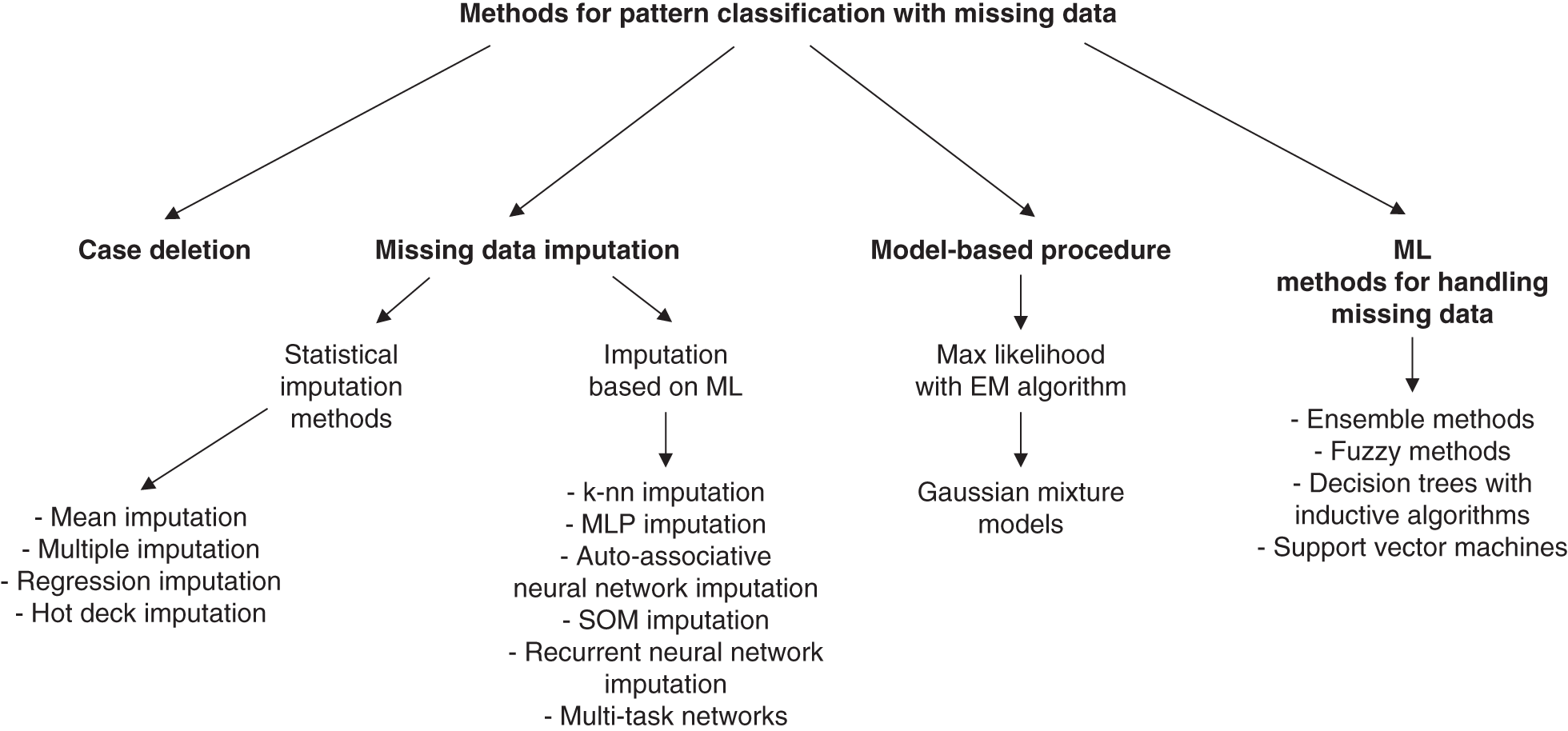
FIGURE 7.6 Methods for pattern classification with missing data. This scheme shows the different procedures that are analyzed in Garcia-Laencina et al. (2010).
Source: Adapted from Garcia-Laencina et al. (2010).
They assess all these methods by comparing mean classification errors across 20 simulated datasets over varying amounts of missingness along with a real medical dataset pertaining to thyroid disease.
Of the machine learning methods used for imputation, they find, similar to Luengo et al. (2012), that it is very much a case of “horses for courses” with different methods performing better in different classification domains, as can be seen in Figures 7.7, 7.8, and 7.9. They conclude that, generally, there is not a unique solution that provides the best results for each classification domain. Thus in real-life scenarios, a detailed study is required in order to evaluate which missing data estimation can help to enhance the classification accuracy the most.
| Missing data in x1 (%) | Missing data imputation | ||||
| KNN | MLP | SOM | EM | ||
| 5 | 9.21 ± 0.56 | 9.97 ± 0.48 | 9.28 ± 0.84 | 8.29 ± 0.24 | |
| 10 | 10.85 ± 1.06 | 10.86 ± 0.79 | 9.38 ± 0.52 | 9.27 ± 0.54 | |
| 20 | 11.88 ± 1.01 | 11.42 ± 0.44 | 10.63 ± 0.54 | 10.78 ± 0.59 | |
| 30 | 13.50 ± 0.81 | 12.82 ± 0.51 | 13.88 ± 0.67 | 12.69 ± 0.57 | |
| 40 | 14.89 ± 0.49 | 13.72 ± 0.37 | 15.55 ± 0.66 | 13.31 ± 0.56 | |
FIGURE 7.7 Misclassification error rate (mean ± standard deviation from 20 simulations) in a toy problem (for more information on the dataset see Garcia-Laencina et al., 2010) after missing values are estimated using KNN, MLP, SOM, and EM imputation procedures. A neural network with six hidden neurons is used to perform the classification stage.
Source: Based on data from Garcia-Laencina et al. (2010).
| Missing data in x2 (%) | Missing data imputation | ||||
| KNN | MLP | SOM | EM | ||
| 5 | 15.92 ± 1.26 | 15.84 ± 1.13 | 16.32 ± 1.13 | 16.19 ± 0.99 | |
| 10 | 16.88 ± 1.16 | 16.87 ± 1.16 | 16.97 ± 1.18 | 16.85 ± 1.03 | |
| 20 | 18.78 ± 1.29 | 19.09 ± 1.29 | 19.30 ± 1.23 | 19.23 ± 1.12 | |
| 30 | 20.58 ± 1.31 | 20.76 ± 1.34 | 22.04 ± 1.01 | 21.22 ± 1.12 | |
| 40 | 22.61 ± 1.30 | 22.76 ± 1.23 | 24.06 ± 1.29 | 23.11 ± 1.37 | |
FIGURE 7.8 Misclassification error rate (mean ± standard deviation from 20 simulations) in Telugu problem (a well-known Indian vowel recognition problem) after missing values are estimated using KNN, MLP, SOM, and EM imputation procedures. A neural network with 18 hidden neurons is used to perform the classification stage.
Source: Based on data from Garcia-Laencina et al. (2010).
| Missing data imputation | |||||
| KNN | MLP | SOM | EM | ||
| Misclassification error rate (%) | 3.01 ± 0.33 | 3.23 ± 0.31 | 3.49 ± 0.35 | 3.60 ± 0.31 | |
| A neural network with 20 hidden neurons is used to perform the classification stage. | |||||
FIGURE 7.9 Misclassification error rate (mean ± standard deviation from 20 simulations) in sick-thyroid dataset after missing values are estimated using KNN, MLP, SOM, and EM imputation procedures. A neural network with 20 hidden neurons is used to perform the classification stage.
Source: Based on data from Garcia-Laencina et al. (2010).
7.3.3. Grzymala-Busse et al. (2000)
Grzymala-Busse et al. (2000) tests how 9 methods of dealing with missing data affect the accuracy of both naïve and new LERS (Learning from Examples based on Rough Sets) classifiers across 10 different datasets.
The missing data methods used are: most common attribute value; concept most common attribute value; C4.5 based on entropy and splitting the example with missing attribute values to all concepts; method of assigning all possible values of the attribute; method of assigning all possible values of the attribute restricted to the given concept; method of ignoring examples with unknown attribute values; event-covering method; a special LEM2 algorithm; and method of treating missing attribute values as special values. More in-depth details of these methods can be found in the paper itself. They use classification error rates and the Wilcoxon signed rank test to assess which methods perform best over the 10 datasets.
Figures 7.10 and 7.11 show us the error rates of each classifier after imputing values using each of the given methods for each dataset.
| Methods | ||||||||||
| Data file | 1 | 2 | 3 | 4 | 5 | 6 | 7 | 8 | 9 | |
| Breast | 34.62 | 34.62 | 31.5 | 28.52 | 31.88 | 29.24 | 34.97 | 33.92 | 32.52 | |
| Echo | 6.76 | 6.76 | 5.4 | - | - | 6.56 | 6.76 | 6.76 | 6.76 | |
| Hdynet | 29.15 | 31.53 | 22.6 | - | - | 28.41 | 28.82 | 27.91 | 28.41 | |
| Hepatitis | 24.52 | 13.55 | 19.4 | - | - | 18.75 | 16.77 | 18.71 | 19.35 | |
| House | 5.06 | 5.29 | 4.6 | - | - | 4.74 | 4.83 | 5.75 | 6.44 | |
| Im85 | 96.02 | 96.02 | 100 | - | 96.02 | 94.34 | 96.02 | 96.02 | 96.02 | |
| New-o | 5.16 | 4.23 | 6.5 | - | - | 4.9 | 4.69 | 4.23 | 3.76 | |
| Primary | 66.67 | 62.83 | 62 | 41.57 | 47.03 | 66.67 | 64.9 | 69.03 | 67.55 | |
| Soybean | 15.96 | 18.24 | 13.4 | - | 4.1 | 15.41 | 19.87 | 17.26 | 16.94 | |
| Tokt | 31.57 | 31.57 | 26.7 | 32.75 | 32.75 | 32.88 | 32.16 | 33.2 | 32.16 | |
FIGURE 7.10 Error rates of input datasets by using LERS new classification.
Source: Based on data from Grzymala-Busse et al. (2000).
| Methods | |||||||||
| Data file | 1 | 2 | 4 | 5 | 6 | 7 | 8 | 9 | |
| Breast | 49.3 | 52.1 | 46.98 | 47.32 | 48.38 | 52.8 | 52.1 | 47.55 | |
| Echo | 27.03 | 25.68 | - | - | 31.15 | 29.73 | 33.78 | 22.97 | |
| Hdynet | 67.49 | 69.62 | - | - | 65.27 | 69.21 | 56.98 | 61.33 | |
| Hepatitis | 38.06 | 28.39 | - | - | 32.5 | 37.42 | 41.29 | 34.84 | |
| House | 10.11 | 7.13 | - | - | 9.05 | 10.57 | 12.87 | 11.72 | |
| Im85 | 97.01 | 97.01 | - | 97.01 | 94.34 | 97.01 | 97.01 | 97.01 | |
| New-o | 11.74 | 11.74 | - | - | 11.19 | 11.27 | 10.33 | 10.33 | |
| Primary | 83.19 | 77.29 | 53.16 | 60.09 | 81.82 | 80.53 | 82.1 | 79.94 | |
| Soybean | 25.41 | 22.48 | - | 4.86 | 24.06 | 24.1 | 21.82 | 22.15 | |
| Tokt | 63.62 | 63.62 | 62.82 | 62.82 | 64.15 | 63.36 | 63.62 | 63.89 | |
FIGURE 7.11 Error rates of input datasets by using LERS naïve classification.
Source: Based on data from Grzymala-Busse et al. (2000).
Grzymala-Busse et al. first conclude that the new extended LERS classifier is always superior to the naïve one. They then compare the different imputation methods concluding that the C4.5 approach and the method of ignoring examples with missing attribute values are the best methods among all nine approaches, whereas the “most common attribute value” method performs worst. They also find that many methods do not differ from one another significantly.
7.3.4. Zou et al. (2005)
Zou et al. (2005) aims to assess 9 different methods of handling missing data by testing the improvement they give to each of the C4.5 and ELEM2 classifiers across 30 datasets, compared to ignoring data points with missing values. They further come up with meta-attributes for each dataset that are used in a rule-based system (i.e. decision tree) to decide under which circumstances one should use each imputation method over the others.
Similar to the other papers, and as the need for a rule-based system would suggest, there is no “clear winner” in terms of imputation techniques. The efficacy of each very much depends on the type of data and meta attributes of the data. As for their system to select which imputation technique to use, they conclude (after testing on a validation set) that this rule-based system is superior to simply selecting one imputation method for all datasets.
7.3.5. Jerez et al. (2010)
Jerez et al. (2010) tests a variety of imputation techniques to impute missing values on a breast cancer dataset. They compare the performance of different statistical methods, namely, mean, hot deck, and multiple imputation, against machine learning methods, namely, multi-layer perceptrons (MLP), self-organizing maps (SOM) and k-nearest neighbors (KNN). For multiple imputation, a variety of algorithms/software are used; Amelia II (bootstrapping-based EM); WinMICE (multiple imputation by chained equations based); and MI in SAS (Markov chain Monte Carlo based). Performance was measured via the area under the ROC curve (AUC) and the Hosmer-Lemeshow goodness of fit test.
They find that, for this dataset, the machine learning methods were the most suitable for imputation of missing values and led to a significant enhancement of prognosis accuracy compared to imputation methods based on statistical procedures, as can be seen in Figure 7.12. In fact, only the improvements of these methods were deemed statistically significant in predicting breast cancer relapses compared to the method of removing entries with missing values.
| AUC | LD | Mean | Hot-deck | SAS | Amelia | Mice | MLP | KNN | SOM |
| Mean | 0.7151 | 0.7226 | 0.7111 | 0.7216 | 0.7169 | 0.725 | 0.734 | 0.7345 | 0.7331 |
| Std. dev. | 0.0387 | 0.0399 | 0.0456 | 0.0296 | 0.0297 | 0.0301 | 0.0305 | 0.0289 | 0.0296 |
| MSE | 0.0358 | 0.0235 | 0.0324 | 0.0254 | 0.1119 | 0.1119 | 0.024 | 0.0195 | 0.0204 |
FIGURE 7.12 Mean, standard deviation, and MSE values for the AUC (area under the ROC curve) values computed for the control model and for each of the eight imputation methods considered.
Source: Based on data from Jerez et al. (2010).
7.3.6. Farhangfar et al. (2008)
Farhangfar et al. (2008) studies the effect of 5 imputation methods, across 15 datasets at varying levels of artificially induced missingness (MCAR), on 7 classifiers. The imputation techniques tested are: mean imputation, hot deck, naïve Bayes (the latter two methods with a recently proposed imputation framework), and a polytomous regression-based method. The classifiers used are; RIPPER, C4.5, k-nearest-neighbor, support vector machine with polynomial kernel, support vector machine with RBF kernel, and naïve Bayes.
The results show that imputation with the tested methods on average improves classification accuracy when compared to classification without imputation. However, there is no universal best imputation method. They also note a few more general cases in which certain imputation techniques seem to perform best. The analysis of the quality of the imputation with respect to varying amounts of missing data (i.e. between 5% and 50%) shows that all imputation methods, except for the mean imputation, improve classification error for data with more than 10% of missing data. Finally, some classifiers such as C4.5 and naïve Bayes were found to be missing data resistant. In other words, they can produce accurate classification in the presence of missing data while other classifiers such as k-nearest-neighbor, SVMs, and RIPPER benefit from the imputation. As C4.5 and naïve Bayes classifiers were found to be missing data resistant, any missing data imputation actually worsened their performance.
7.3.7. Kang et al. (2013)
Kang et al. (2013) proposes a new single imputation method based on locally linear reconstruction (LLR) that improves the prediction performance of supervised learning (classification and regression) with missing values. They compare the proposed missing value imputation method (LLR) with six well-known single imputation methods – mean imputation; hot deck; KNN; expectation conditional maximization (ECM); mixture of Gaussians (MoG); k-means clustering (KMC) – for different learning algorithms (logistic regression; linear regression; KNN regression/classification; artificial neural networks; decision trees; and the proposed LLR) based on 13 classification and 9 regression datasets, across a variety of amounts of (artificially induced) missing data.
Kang claims that: (1) all imputation methods helped to improve the prediction accuracy compared to removing data points with missing values, although some were very simple; (2) the proposed LLR imputation method enhanced the modeling performance more than all other imputation methods, irrespective of the learning algorithms and the missing ratios; and (3) LLR was outstanding when the missing ratio was relatively high and its prediction accuracy was similar to that of the complete dataset.
7.4. SUMMARY
As we have seen, each of the previous 7 papers draws different, and in some cases conflicting, conclusions about a variety of imputation techniques. Aside from LLR in Kang (2013), most methods are deemed to be superior in certain situations and not in others. As such, the general consensus seems to be that there is no clear choice of imputation technique that outperforms all others, other than possibly LLR. Due to the lack of papers reporting on LLR's use for data imputation, though, we are hesitant to categorically state it as the imputation technique of choice, rather than suggest trying a variety of methods based on the particulars of the dataset at hand. Hence, it is most likely that, as with all machine learning algorithms, each has its own benefits and drawbacks. Hence, there is no one algorithm that works in all cases in line with the no-free-lunch theorem.
The literature review in this chapter is by no means exhaustive. It can also be the case that none of these algorithms is applicable for alternative data treatment where, for example, spatial information (e.g. satellite images) can be important to use. We will show how to apply spectral techniques in this case in the next chapter. Also, time series could contain important temporal information that can be leveraged. Again, we will show a case study in the next chapter where information about the temporal ordering is used for the imputation.
NOTES
- 1 See Little (2019).
- 2 In any application, a judgment on whether we will lose a lot or a small amount of data depends on the aim of the application. In the case study in the next chapter, the data can be used for the calculation of the Expected Shortfall (ES), for example. The calculation of ES requires recent and plentiful data, which induces a low tolerance to long streaks of missing data.
- 3 The reader can also take a look at Graham (2009), who provides an exhaustive introduction to missing data problems.
- 4 See Section 4.1 in Luengo et al. (2012).