
CHAPTER 4
Machine Learning Techniques
4.1. INTRODUCTION
In this chapter, we will discuss several topics centered on machine learning. The rationale behind discussing it is that machine learning can be an important part of utilizing alternative data within the investment environment. One particular usage of machine learning concerns structuring the data, which is often a key step in the investment process. Machine learning can also be used to help create forecasts using regressions, such as for economic data or prices, using various factors, which can be drawn from more traditional datasets, such as market data and also alternative data. We can also use techniques from machine learning for classification, which can be useful to help us model various market regimes.
To begin with, we give a brief discussion concerning the variance-bias trade-off and the use of cross-validation. We talk about the three broad types of machine learning, namely supervised, unsupervised, and reinforcement learning.
Then we have a brief survey of some of the machine learning techniques that have applications to alternative data. Our discussion of the techniques will be succinct, and we will refer to other texts as appropriate. We begin with relatively simple cases from supervised machine learning, such as linear and logistic regression. We move on to unsupervised techniques. There is also a discussion of the various software libraries that can be used such as TensorFlow and scikit-learn.
The latter part of the chapter addresses some of the particular challenges associated with machine learning. We give several use cases in financial markets, and which machine learning techniques could be used to solve them, ranging from forecasting volatility to entity matching. We talk about the difficulties that arise when using it with financial time series, which are by nature nonstationary. We also give practical use cases on how to structure images and also text, through natural language processing.
4.2. MACHINE LEARNING: DEFINITIONS AND TECHNIQUES
4.2.1. Bias, Variance, and Noise
This section discusses one of the most important trade-offs that must be considered when building a machine learning model. This trade-off is general and arises regardless of the domain and the task we are focused on. While it is methodological in nature, there are also additional trade-offs between methodology, technology, and business requirements. We will touch upon those in Section 4.4.4. What we can say at this point is that the choices we make here in regard to this trade-off can significantly impact on our investment strategy.
Imagine that we have a dataset ![]() and want to model the relationship
and want to model the relationship ![]() with
with ![]() . As pointed out by Lopez de Prado (2018)1 models generally suffer from three errors: bias, variance, and noise, which jointly contribute to the total output error. More specifically:
. As pointed out by Lopez de Prado (2018)1 models generally suffer from three errors: bias, variance, and noise, which jointly contribute to the total output error. More specifically:
- Bias: This error is caused by unrealistic and simplifying assumptions. When bias is high, this means that the model has failed to recognize important relations between features and outcomes. An example of this is trying a linear fit on data whose data-generating process is nonlinear (e.g. quadratic). In this case, the algorithm is said to be “underfit.”
- Noise: This error is caused by the variance of the observed values, like changes to external variables to the dataset or measurement errors. This error is irreducible and cannot be explained by any model.
- Variance: This error is caused by the sensitivity of the model predictions to small changes in the training set. When the variance is high, this means that the algorithm has overfit the training set. Therefore, even minuscule changes in the training set can produce wildly different predictions – for example, fitting a polynomial of degree four to data generated by a quadratic data-generating process. Ultimately, rather than modeling the general patterns in the training set, the algorithm has mistaken the noise for signal. Hence, it was fit to the noise, rather than the underlying signal.
We can express this in mathematical terms as follows. Assume the data-generating process (unknown) is given by ![]() with
with ![]() and
and ![]() .
. ![]() is what we have to estimate. Let's denote by
is what we have to estimate. Let's denote by ![]() our estimate. The expected error of the fit by the function
our estimate. The expected error of the fit by the function ![]() at the point
at the point ![]() is given by:
is given by:
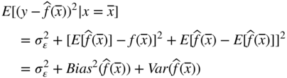
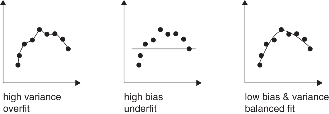
FIGURE 4.1 Balance between high bias and high variance.
Source: Based on data from Towards Data Science (https://towardsdatascience.com/understanding-the-bias-variance-tradeoff-165e6942b229).
Typically, the bias decreases as model complexity2 increases. The variance, on the other hand, increases.3 If we assume that the data we are modeling is stationary over the training and test periods, then our aim will be to minimize the expected error of the fit (e.g. when trying to forecast asset returns). This error will then be an interplay between variance and bias and will be influenced by the complexity of the model we choose, as Equation 4.1 shows. Hence, we want to strike a balance between bias and variance. We don't want a model that has high bias or high variance (see Figure 4.1).
Of course, most of the time we will be (hopefully!) making models assumptions rooted in economic theory that will limit the model space, and hence typically reduce the model complexity. Other times we will make sacrifices, such as when required to deliver the results of a calculation on an unstructured dataset quickly and on a device that is slow, for example, a mobile phone – in this case a simpler model could be preferred but we should always keep in mind the trade-off of this section. In essence, we want to make the model simple enough to model what we want, but no simpler.
4.2.2. Cross-Validation
Cross-validation (CV) is a standard practice to determine the generalization capability of an algorithm. When calibrated on a training set it can yield very good fits but out-of-sample its performance can be drastically reduced. In fact, as Lopez de Prado (2018) argues, ML algorithms calibrated on a training set “are no different from file lossy-compression algorithms: They can summarize the data with extreme fidelity, yet with zero forecasting power.” Lopez de Prado also argues that CV fails in finance as it is far-fetched to assume that the observations in the training and validation set are i.i.d. (independent and identically distributed). This could happen, for example, due to leakage when training and validation sets contain the same information.
In general, CV is also used for the choice of parameters of a model in order to maximize its out-of-sample predictive power. We do not want to fit parameters that happen to simply work in a very short and specific historical period at the cost of poor out-of-sample performance.
For the purposes of an investment strategy, our CV will be determined by the backtesting method, where we specifically leave some historical data for out-of-sample testing. We discussed backtesting methodology in Section 2.5. We will also discuss it again in great length in Chapter 10, and in many of the later use cases in the book. We note that while backtesting has the general flavor of a CV method, it is not subject, at least to the same degree, to the criticisms made earlier. By design, it can better handle non-i.i.d. data, which is what we need.
4.2.3. Introducing Machine Learning
We have already mentioned machine learning a number of times in the text, with reference to many areas of relevance for alternative data, such as structuring datasets and anomaly detection. In the next few sections of the book, we give an introductory look at machine learning and discuss some of the most popular techniques used in this area. Later, we delve into more advanced techniques such as neural networks.
All of machine learning can be split into one of three groups: supervised learning, unsupervised learning, and reinforcement learning. In all types of machine learning, however, we are trying to maximize some score function (or minimize some loss function), whether this is a likelihood (from classical statistics) or some other objective function.
4.2.3.1. Supervised Learning
In supervised learning, for each data point, we have a vector of input variables, ![]() , and a vector of output variables,
, and a vector of output variables, ![]() , forming a set of
, forming a set of ![]() pairs. The aim is to try to predict
pairs. The aim is to try to predict ![]() by using
by using ![]() .4 Within this predictive branch of supervised learning, there are two streams: regression and classification. Regression consists of trying to predict a continuous variable, such as
.4 Within this predictive branch of supervised learning, there are two streams: regression and classification. Regression consists of trying to predict a continuous variable, such as ![]() . An example might be predicting a stock's returns using the current interest rate,
. An example might be predicting a stock's returns using the current interest rate, ![]() , and a momentum indicator for the stock,
, and a momentum indicator for the stock, ![]() . For classification, we predict which group something belongs in, such as
. For classification, we predict which group something belongs in, such as ![]() . An example might be trying to predict whether a mortgage will default (belongs to class
. An example might be trying to predict whether a mortgage will default (belongs to class ![]() ) given the recipient's credit score,
) given the recipient's credit score, ![]() , and the current mortgage interest rate,
, and the current mortgage interest rate, ![]() .
.
Classification problems are then further subdivided into two categories, generative and discriminative. Generative algorithms provide us with probabilities that the inputs belong to each class, such as ![]() and interest rate of
and interest rate of ![]() . We must then decide how to use these probabilities to assign classes.5 Discriminative algorithms merely assign a class to each of the input vectors.
. We must then decide how to use these probabilities to assign classes.5 Discriminative algorithms merely assign a class to each of the input vectors.
In Chapter 14, for example, we use supervised learning in the form of a linear regression to fit earnings per share estimates with various alternative datasets, such as location data and news sentiment for specific US retailers.
4.2.3.2. Unsupervised Learning
Rather than trying to predict the data, unsupervised learning is about understanding and augmenting the data. Here, instead of having ![]() pairs, we simply have
pairs, we simply have ![]() vectors (i.e. there is nothing to predict). Outputs of unsupervised learning can often be good inputs to supervised learning models. Among the many subfields of unsupervised learning, the most popular are probably clustering and dimensionality reduction. Clustering is about grouping data points, but without prior knowledge of what those groups might be, whereas dimensionality reduction is about expressing the data using fewer dimensions.
vectors (i.e. there is nothing to predict). Outputs of unsupervised learning can often be good inputs to supervised learning models. Among the many subfields of unsupervised learning, the most popular are probably clustering and dimensionality reduction. Clustering is about grouping data points, but without prior knowledge of what those groups might be, whereas dimensionality reduction is about expressing the data using fewer dimensions.
A common example of clustering is in assigning stocks to sectors. This is particularly useful for diversification because it may not be particularly obvious at first that a stock should belong to a sector. By understanding how the elements of our universe form groups (i.e. sectors) we can ensure we don't give any one group too much weight within our portfolio.
4.2.3.3. Reinforcement Learning
For reinforcement learning, rather than map an input vector, ![]() , to a known output vector that denotes some variable,
, to a known output vector that denotes some variable, ![]() , either continuous or categorical, we instead want to map an input vector to an action. This is done without prior knowledge of which input vectors we want to map to which actions. These actions then lead to some reward, either immediately or later down the line, decided by some rule set or “environment.”
, either continuous or categorical, we instead want to map an input vector to an action. This is done without prior knowledge of which input vectors we want to map to which actions. These actions then lead to some reward, either immediately or later down the line, decided by some rule set or “environment.”
If supervised learning is deciding which stocks will experience positive returns (which we would then decide to buy), then reinforcement learning is about teaching the model which stocks to buy (without explicitly stating so) by allowing it to learn that buying stocks that experience positive returns is a good thing. One way to do this is perhaps by giving it a “reward” proportional to end-of-day P&L and reinforcement learning, therefore, could be useful to derive trading strategies themselves, rather than us building the strategies around fixed rules where the inputs to those strategies come from models.
The difficulty with reinforcement learning is that, because our model starts off as being “dumb” and we often have many choices we could make at any point in time, it requires a very large amount of data to train, likely more than currently exists for any financial market. One way to overcome this is if we could set up a way to artificially generate real enough financial market simulations to allow the model to learn what to do in certain situations, much like how we can simulate games of chess or Go. Doing this, however, is not so simple, although there have been some attempts to address this problem in finance.
Reinforcement learning looks like it could be extremely powerful when applied to finance; however, at present, we are at very early stages. As such, we don't discuss reinforcement learning further in this text. For readers interested in methods of creating synthetic financial data, Pardo (2019) discusses the use of GANs (generative adversarial networks) to create such datasets. It shows how to create financial time series that exhibit similar characteristics to existing time series. For example, it shows how to create many synthetic time series that have similar behavior to the popular VIX index.
4.2.4. Popular Supervised Machine Learning Techniques
4.2.4.1. Linear Regression
Linear regression is probably the first model one should learn in one's attempt to expose oneself to machine learning. It is remarkably simple to understand, quick to implement, and, in many cases, extremely effective. Before attempting any other more complicated model, one should probably attempt a linear model first. This is also our approach in the use case chapters.
Linear regression, unsurprisingly, assumes a linear relationship between the dependent variable, ![]() , and the explanatory variables,
, and the explanatory variables, ![]() . In particular, the model is usually denoted
. In particular, the model is usually denoted ![]() or
or ![]() with
with ![]() augmented to include an element that is always
augmented to include an element that is always ![]() to represent the intercept
to represent the intercept ![]() , and
, and ![]() the error term.6 In linear regression we are attempting to minimize the sum of the squared errors,
the error term.6 In linear regression we are attempting to minimize the sum of the squared errors, ![]() (i.e. OLS, ordinary least squares) – see Figure 4.2 for an example.
(i.e. OLS, ordinary least squares) – see Figure 4.2 for an example.
Other than linearity, we further assume that:
- The errors,
 , are:
- Normally distributed with mean zero, and
- Homoscedastic (all having the same variance)
- There is no (or suitably small) multicollinearity between the
 , and
, and - Errors have no autocorrelation – knowledge of the previous error should not give any information about the next error.
Violations of these assumptions can lead to very strange results. It is, therefore, worth doing some quick checks beforehand to see if they seem to be roughly met. Variations, such as ridge regression, instead minimize a penalized version of the sum of squared errors. This approach is less susceptible to overfitting based on outlying points, making the model less complex, and also deals with some of the problems of multicollinearity between the various ![]() .
.
Linear regression is often used in finance in the modeling of financial time series, given that we often have only small datasets for learning parameters. This is particularly the case if we are limited to using daily or lower-frequency data. This contrasts to techniques such as neural networks, which have many more parameters and hence need much more training data to learn these parameters. Another benefit of linear regressions is that we can often more easily explain the output (within reason, provided there are not too many variables).
This ability to explain the output of a model is important in areas such as finance, particularly if we are trying to do higher-level tasks, such as generate a trading signal. It tends to be less important where we are trying to automate relatively manual tasks, where we can more readily explain a “ground truth.” These can include cleaning a dataset or doing natural language processing on a text.
For an example of how linear regression can be used specifically for alternative data models, see Chapter 10, where we use it to create trading strategies for automotive stocks, based on traditional equity ratios and also an alternative dataset based on automotive supply chains. Linear regression is also used in many other instances in this book, to help model estimates such as earnings per share, using input variables such as physical customer traffic data derived from location data (see Chapter 14), and using input variables like retailer car park counts derived from satellite imagery (see Chapter 13).
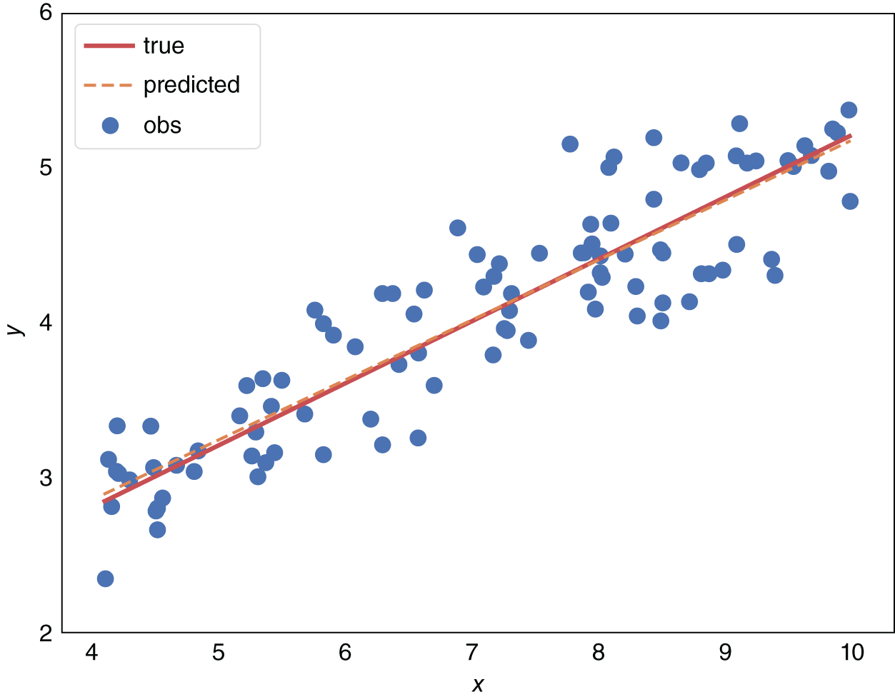
FIGURE 4.2 Visualizing linear regression.
4.2.4.2. Logistic Regression
Logistic regression is to classification what linear regression is to regression. It is, therefore, one of the first machine learning methods one should learn. Like linear regression, logistic regression takes a set of inputs and combines them in a linear fashion to get an output value. If this output value is above some threshold, we classify those inputs as group ![]() and otherwise as group
and otherwise as group ![]() (see Figure 4.3). As doing things on a linear scale is slightly confusing, logistic regression converts this linear value to a probability through the use of the logistic function,
(see Figure 4.3). As doing things on a linear scale is slightly confusing, logistic regression converts this linear value to a probability through the use of the logistic function, ![]() .
.
Putting this all together, we calculate the probability that the inputs belong to group![]() by calculating
by calculating ![]() , or
, or ![]() , and classify the inputs to group
, and classify the inputs to group ![]() if
if ![]() and to group
and to group ![]() otherwise.7 Similar to linear regression, logistic regression assumes that there is little to no multicollinearity between the
otherwise.7 Similar to linear regression, logistic regression assumes that there is little to no multicollinearity between the ![]() . However, as we apply a nonlinear transformation here, instead of requiring a linear relationship between the
. However, as we apply a nonlinear transformation here, instead of requiring a linear relationship between the ![]() and
and ![]() , we instead require a linear relationship between the
, we instead require a linear relationship between the ![]() and
and ![]() , the log-odds. The only strict constraint is that an increase in each of the features should always lead to an increase/decrease in the probability of belonging to a class (i.e. increase always causes increase or increase always causes decrease). Like linear regression, logistic regression is likely the first model one should attempt when trying to classify something based on just a few inputs (i.e. not performing something like image classification, although it is possible in theory).
, the log-odds. The only strict constraint is that an increase in each of the features should always lead to an increase/decrease in the probability of belonging to a class (i.e. increase always causes increase or increase always causes decrease). Like linear regression, logistic regression is likely the first model one should attempt when trying to classify something based on just a few inputs (i.e. not performing something like image classification, although it is possible in theory).
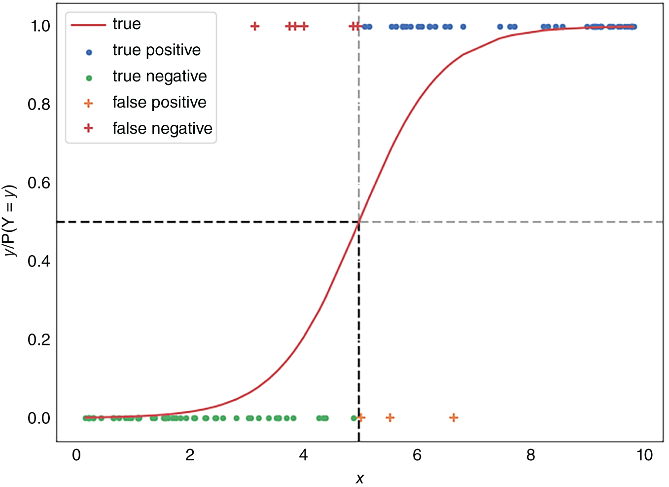
FIGURE 4.3 Visualizing logistic regression.
Logistic regression could be used in a variety of situations within finance. Some obvious areas could include classification of different market regimes. We could seek to create a model to classify if markets were ranging or trending. Typical inputs of such a model could include price data for the asset we were seeking to identify and also volatility. Typically, lower levels of volatility are related to ranging markets while increasing levels of volatility tend to be an indication of trend. A simple approach could be used to identify the various risk regimes of a market, using various risk factors as inputs. These risk factors could include credit spreads, implied volatility across various markets, and so on. We could also include alternative datasets such as news volume or readership figures. For example, in Chapter 15, we discuss how news volume can be a useful indicator to model market volatility and we also give specific examples around macroeconomic events like FOMC meetings.
4.2.4.3. Softmax Regression
Although powerful, logistic regression, in the form described above, does not handle the case of multiple classes. Say we want to predict whether a stock will experience returns below ![]() , from
, from ![]() to
to ![]() , or above
, or above ![]() . How do we handle this with logistic regression? This is where softmax regression (aka multinomial logistic regression) comes in. We won't get into the mathematics of why softmax regression is the natural extension of logistic regression, but simply state its formula. In softmax regression, for
. How do we handle this with logistic regression? This is where softmax regression (aka multinomial logistic regression) comes in. We won't get into the mathematics of why softmax regression is the natural extension of logistic regression, but simply state its formula. In softmax regression, for ![]() classes, we take:
classes, we take:
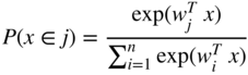
This allows us to predict the class of something in a very similar fashion to logistic regression, only this time with more than two classes. Here it is common to take the class with the highest “probability” as what we classify the inputs to.
4.2.4.4. Decision Trees
Unlike previously mentioned methods, decision trees can be used for both classification and regression. Essentially, decision trees boil down to a series of decisions, such as “Is![]() ?” The results of these decisions instruct us on which branch of the tree to follow, left or right. In this way, we can arrive at a set of leaves at the end of our tree. These leaves can feed either to a class (i.e. classify something) or to a continuous variable (i.e. regress something).8 Generally, for regression, the leaf node
?” The results of these decisions instruct us on which branch of the tree to follow, left or right. In this way, we can arrive at a set of leaves at the end of our tree. These leaves can feed either to a class (i.e. classify something) or to a continuous variable (i.e. regress something).8 Generally, for regression, the leaf node ![]() outputs the average value of the dependent variable for all data points that pass the set of rules to arrive at leaf
outputs the average value of the dependent variable for all data points that pass the set of rules to arrive at leaf ![]() . Because of their structure, decision trees can easily take in both categorical and continuous variables as inputs. Furthermore, decision trees have none of the linearity assumptions that linear and logistic regression have. Finally, they automatically perform what we call feature selection through their training. After we have trained our model, there may be features that are not used in our tree, an indication that these features are unnecessary.
. Because of their structure, decision trees can easily take in both categorical and continuous variables as inputs. Furthermore, decision trees have none of the linearity assumptions that linear and logistic regression have. Finally, they automatically perform what we call feature selection through their training. After we have trained our model, there may be features that are not used in our tree, an indication that these features are unnecessary.
4.2.4.5. Random Forests
Random forests are an extension of decision trees that make use of the “wisdom of the crowd” mantra, similar to the efficient market hypothesis. Although each individual decision tree is often not particularly performant in itself, if we can train lots of them, their average probably is, assuming we don't just have all trees predicting the same thing. To achieve this, we first perform what is called bagging. Bagging consists of training on only a random subset of the available data. This leads to different trees through different training sets. To further arrive at different trees, instead of randomly selecting data for each tree, at each new node, we only allow the algorithm to select from a random subset of the available features when deciding which to make a split on. This stops all trees deciding to split on, say, ![]() first, thus leading to an even more diverse set of trees. Finally, now that we have a group of, hopefully, different trees, we take their average prediction as our overall prediction. This group of trees is our random forest. For a use case of random forests in filling missing values in the case of time series data, see Chapter 7.
first, thus leading to an even more diverse set of trees. Finally, now that we have a group of, hopefully, different trees, we take their average prediction as our overall prediction. This group of trees is our random forest. For a use case of random forests in filling missing values in the case of time series data, see Chapter 7.
4.2.4.6. Support Vector Machines
Support vector machines (SVMs) essentially boil down to finding a line (hyperplane) that best separates two different classes of data points. In fact, SVMs are very similar to logistic regression in this sense. Where they differ, however, is how this is achieved. Logistic regression trains to maximize the likelihood of the sample. SVMs train to maximize the distance between the decision boundary (line/hyperplane) and the data points. Figure 4.4 shows an example of a decision boundary in black along with the distance of the nearest points for each class. Obviously, this cannot always be done by a straight line. If we would like to create a model to classify different market regimes, SVM can be considered as an alternative to using logistic regression, which has historically been used for such models.
An important point is that logistic regression is more sensitive to outliers than SVM due to the loss function used. Note that it isn't always the case that having less sensitivity to outliers is advantageous.
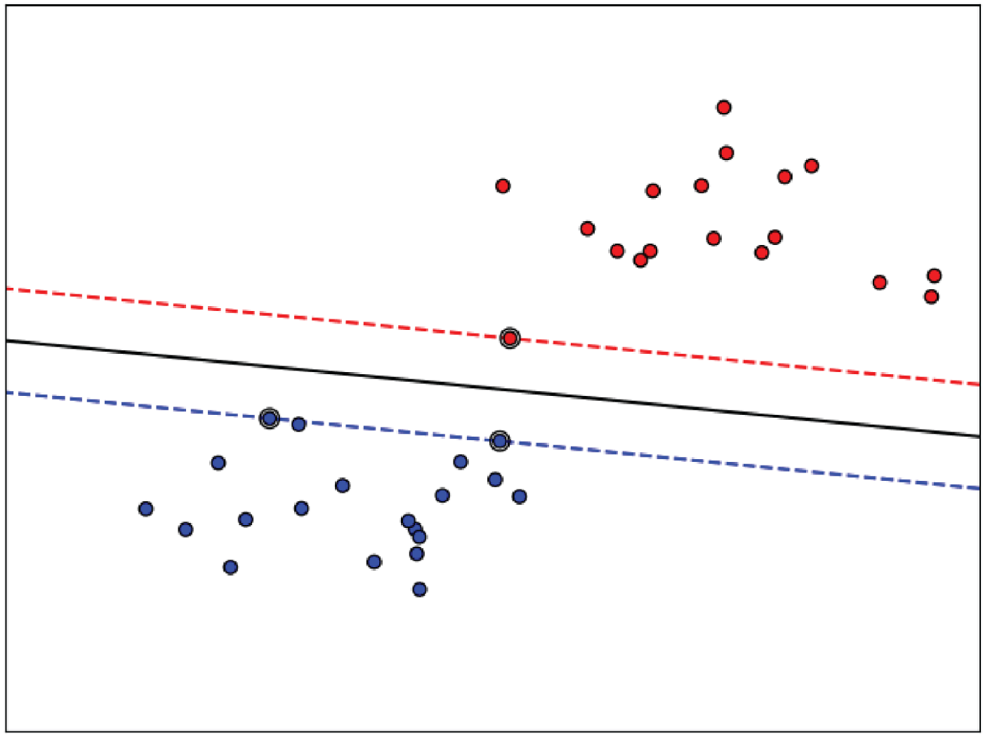
FIGURE 4.4 SVM example: The black line is the decision boundary.
While logistic regression outputs a probability of belonging to each class (it is generative), SVMs simply classify each data point (they are discriminative) and so we don't get a sense of whether data points were “obviously” in a class, such as ![]() , or somewhere between two classes (on the border), such as
, or somewhere between two classes (on the border), such as ![]() .
.
A benefit of SVMs, however, comes in how they deal with nonlinear relationships. Since their invention in 1963, mathematicians came up with the “kernel trick” so that SVMs can support nonlinear decision boundaries. Generally, a kernel is used to embed the data in a higher-dimensional space. In this new space, we may be able to find a linear decision boundary, after which we can transform back to the original space, resulting in a nonlinear decision boundary. In Figure 4.5, we illustrate the kernel trick. We first present a two-dimensional space. We can see that it is difficult to separate the two clusters from drawing a straight line. By converting to a higher-dimensional space, in this case of dimension three, we find that it is now possible to separate out the points with a linear hyperplane.
SVMs have been shown to perform well for image classification. While they do not perform as well as CNNs9 when there is a large amount of training data at hand (e.g. for image recognition), for smaller datasets they tend to outperform them.
4.2.4.7. Naïve Bayes
The final supervised learning method we will mention is naïve Bayes. Naïve Bayes is a classification algorithm that uses the critical assumption that the value of each feature, ![]() , is independent of the value of any other feature,
, is independent of the value of any other feature, ![]() , given the class variable,
, given the class variable, ![]() .
.
Using Bayes' theorem, we have that:

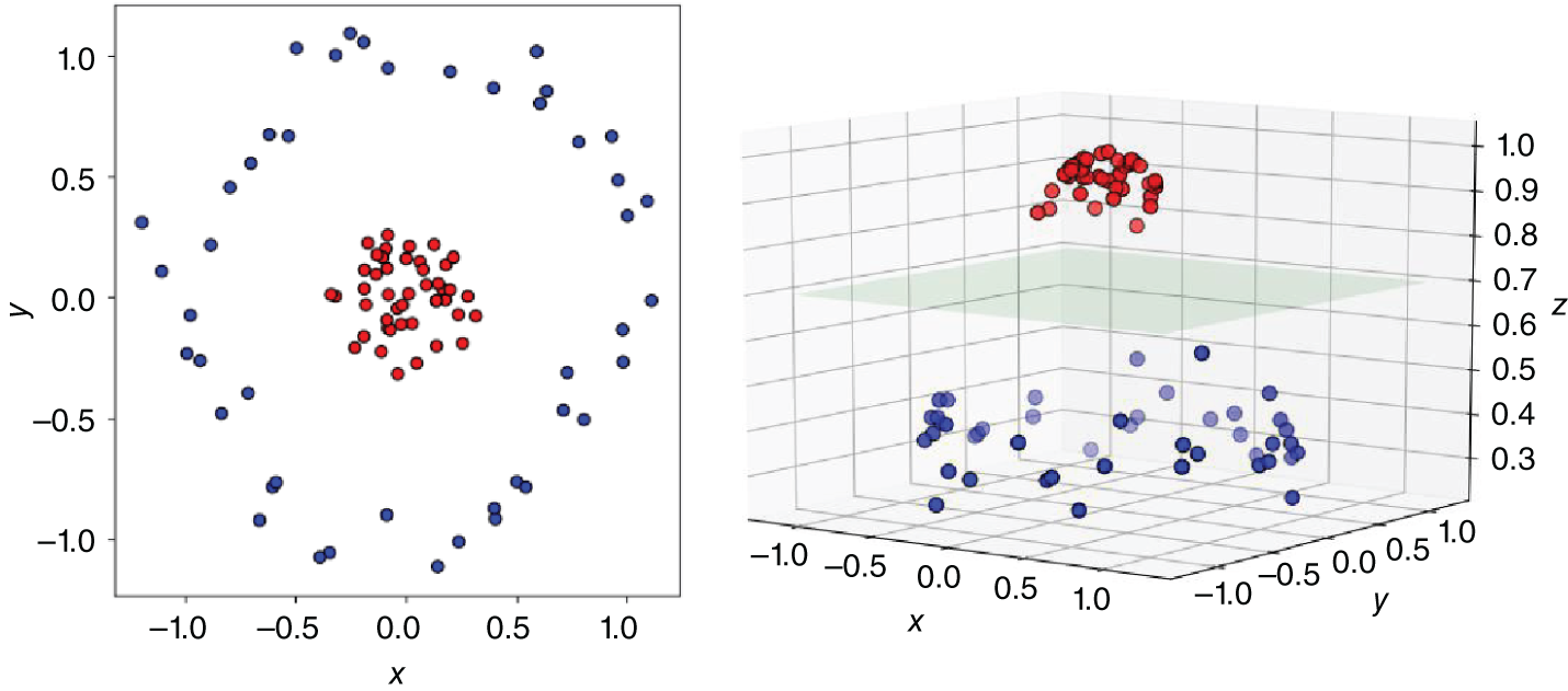
FIGURE 4.5 Kernel trick example.
In this formula the following assumption was made:
(i.e. the features are independent given the class ![]() ). There is not a single algorithm for training naïve Bayes classifiers, but rather a family of algorithms based on the aforementioned assumption.
). There is not a single algorithm for training naïve Bayes classifiers, but rather a family of algorithms based on the aforementioned assumption.
If the assumption of naïve Bayes is satisfied, it generally performs very well; however, it still can perform well if it is violated. Naïve Bayes often only requires a small amount of data to train on; however, given enough data, it is often surpassed in its predictive ability by other methods, such as random forests.
Naïve Bayes has been shown to be useful for natural language processing and, therefore, can be useful for sentiment analysis. We discuss natural language processing in more detail in Section 4.6.
4.2.5. Clustering-Based Unsupervised Machine Learning Techniques
4.2.5.1. K-Means
K-means attempts to group data points into ![]() groups/clusters. Essentially it randomly assigns
groups/clusters. Essentially it randomly assigns ![]() “means” in our data, groups each data point to a “mean” via some distance function, and recalculates the mean of each group. It iterates this process of assigning data points to a group/mean and recalculating mean locations until there is no change. As new data points arrive, we can, therefore, assign them to one of these groups. K-means is used in Chapter 7 to describe the missingness patterns within the data. We also use it in Chapter 9, in a case study based on Fed communication events. There, we find that K-means is particularly effective in identifying outliers in among the various Fed communication events.
“means” in our data, groups each data point to a “mean” via some distance function, and recalculates the mean of each group. It iterates this process of assigning data points to a group/mean and recalculating mean locations until there is no change. As new data points arrive, we can, therefore, assign them to one of these groups. K-means is used in Chapter 7 to describe the missingness patterns within the data. We also use it in Chapter 9, in a case study based on Fed communication events. There, we find that K-means is particularly effective in identifying outliers in among the various Fed communication events.
As with other clustering algorithms, it also has applicability for identifying similar groups of stocks. As we noted earlier in this chapter, typically, stocks tend to be grouped together based on sectors that have been picked by experts. However, in practice, when using clustering algorithms based on their price moves, we might discover dependencies between stocks that are not necessarily explained by such sector classifications. Furthermore, such approaches are far more dynamic than arbitrary sector classifications, which rarely change over time.
4.2.5.2. Hierarchical Clustering
Rather than assume centroids/means for clusters, hierarchical cluster analysis (HCA) assumes either that all data points are their own cluster, or that all data points are in one cluster. It moves between these two extremes, adding or removing to the clusters based on some notion of distance. An example might be to start with all data points in separate clusters, linking them together according to whichever data point/cluster is nearest to another. This continues this until one ends up with one large cluster. This way one can have any number of clusters ![]() according to the hierarchy one builds by linking clusters together.
according to the hierarchy one builds by linking clusters together.
If we think of portfolio optimization, Markovitz's critical line approach uses optimization based on forecasted returns, which is hard to estimate. The results can often be quite unstable and can sometimes concentrate risk in a specific asset. Risk parity, on the other hand, doesn't use covariance, and instead weights assets by the inverse of their volatility.
Instead, hierarchical clustering can be used in portfolio construction. Lopez de Prado (2018) introduces the hierarchical risk parity approach in order to do asset allocation and avoids the use of forecasted returns. It doesn't require having to invert a covariance matrix, but instead uses the covariance matrix to create clusters, and then diversifies the portfolio weights between the various clusters.
4.2.6. Other Unsupervised Machine Learning Techniques
Other than clustering, there are many other ways in which we can explore our unlabeled data.
4.2.6.1. Principle Component Analysis
Principle component analysis (PCA) consists of trying to find a new set of orthogonal axes for our data, with each successive axis explaining less of the variance than the previous. By doing this, we can select a small subset of our new axes to use while still being able to explain the majority of the variance in the data. PCA can, therefore, be seen as a sort of compression algorithm. One example of PCA within finance is in interest rate swaps (IRSs) where the first three principal components explain the level, slope, and curvature of the IRS curve, typically explaining 90–99% of the variance. Singular value decomposition, an extension of PCA called singular value decomposition (SVD), is used in Chapter 8 to reconstruct time series and images with missing points.
4.2.6.2. Autoencoders
Although we don't describe them fully now, autoencoders are similar to PCA in that they allow us to express our data via a different representation (encoding) and are typically used for dimensionality reduction. They are also useful in allowing models to learn which combinations of categorical inputs are similar. For more information on autoencoders, see Section 4.2.8.
4.2.7. Machine Learning Libraries
In this section, we describe two of the most popular machine learning libraries that we also use for the use cases we will explore later.
4.2.7.1. scikit-learn
The absolute go-to machine learning Python library for almost all of the above methods is scikit-learn. It offers a high-level API for a plethora of the most popular machine learning algorithms also offering preprocessing and model selection capabilities.
4.2.7.2. glmnet
As the name would suggest, glmnet is used for running general linear models. Originally written for the R programming language, there are now both Python and Matlab ports. It offers methods to train linear, logistic, multinomial, Poisson, and Cox regression models. It has a more statistics-focused set of algorithms than scikit-learn, offering ![]() values and such for trained models.
values and such for trained models.
4.2.8. Neutral Networks and Deep Learning
Now that we have been introduced to the basics of machine learning, let us discuss the current hot topic, neural networks. They have many applications, especially when dealing with unstructured data, which is essentially most of the alternative data world. Roughly speaking, a neural network is a collection of nodes (aka neurons), weights (slopes), biases (intercepts), directed edges (arrows), and activation functions. The nodes are sorted into layers, typically with an input layer, ![]() hidden layers, and an output layer. For every layer other than the input layer, each node has nodes from previous layers fed into it (via the directed edges), each of which is multiplied by some weight, summed together and added to a bias.10 The node output is generated by applying an activation function to this weighted sum.
hidden layers, and an output layer. For every layer other than the input layer, each node has nodes from previous layers fed into it (via the directed edges), each of which is multiplied by some weight, summed together and added to a bias.10 The node output is generated by applying an activation function to this weighted sum.
Ultimately, we need to fit the various parameters of the neural network to the data. As with other machine learning techniques, this involves selecting a set of weights and bias in order to minimize a loss function. The first step is to randomly initialize the various weights of the model. We can then do forward propagation, to compute the node output from the inputs and randomized parameters. The output from this randomized model is then compared to the actual output we want by computing the loss function. In the context of a trading strategy, our model output could be the returns.
The next step is to select new weights, so that we can reduce the loss function. We could attempt to do this by brute force. However, this is typically not feasible given the number of parameters in many neural networks. Instead, we take the derivative of the loss function to understand this will give us the sensitivity of the various weights with respect to the loss function. We can then backpropagate the loss from the loss at the output to the input nodes. The next step is to update the weights, depending on the sign of the derivative. If the derivative is positive, it means that making the weight greater will increase the error, hence we need to reduce the size of that weight. Conversely, a negative derivative implies we should make the weight greater.
We then loop back to the beginning and start again, with our new updated weights, rather than the randomized weights. This exercise is repeated till our model converges to an acceptable tolerance. The learning rate will govern how much we “bump” the weight. The step size needs to be sufficiently small for the search not to skip over local optima. However, if the step size is too small, it will be computationally more expensive to find a solution, given that we will end up doing many more loops.
We shall now follow with some examples of neural networks, and also how to represent other statistical models like linear regressions as neural networks.
4.2.8.1. Introductory Examples
4.2.8.1.1. Linear regression as a neural network In Figure 4.6 we have an input layer, an output layer, and no hidden layers. We have 2 nodes in our input layer, ![]() and
and ![]() , and
, and ![]() node in our output layer,
node in our output layer,![]() . For the output layer, each node in the previous layer (here our input layer) has an associated weight,
. For the output layer, each node in the previous layer (here our input layer) has an associated weight, ![]() and
and ![]() . We also have a bias,
. We also have a bias, ![]() . To “feed forward” from our input layer to our output layer, we multiply each input by its weight, sum all the results together, and add on the bias. In the case of Figure 4.2 we, therefore, have
. To “feed forward” from our input layer to our output layer, we multiply each input by its weight, sum all the results together, and add on the bias. In the case of Figure 4.2 we, therefore, have ![]() , or
, or ![]() , our standard linear regression equation.
, our standard linear regression equation.
4.2.8.1.2. Single class logistic regression as a neural network You may notice that we originally mentioned activation functions, but we have not used them so far. To illustrate the use of an activation function, we now demonstrate logistic regression. Similar to before, we have ![]() input nodes and
input nodes and ![]() output node (see Figure 4.7). Here, however, instead of the output node having an associated bias and weights for the previous layer, it now also has an associated activation function,
output node (see Figure 4.7). Here, however, instead of the output node having an associated bias and weights for the previous layer, it now also has an associated activation function, ![]() , the logistic (also known as the expit) function, with
, the logistic (also known as the expit) function, with ![]() . Here, the equation becomes
. Here, the equation becomes ![]() , or
, or ![]() , the standard logistic regression equation. We could say then that previously we used the identity function
, the standard logistic regression equation. We could say then that previously we used the identity function ![]() as the activation function.
as the activation function.
4.2.8.1.3. Softmax regression as a neural network Finally, we now show multi-class logistic regression (see Figure 4.8). Notice here that each node on the input layer now has two weights associated with it, each pertaining to a different node in the next layer. This is why it makes more sense to think of the weights as “belonging” to the node they feed into (and storing them in a vector). For the activation functions, however, they are all the same across this layer, ![]() , as is usually the case. From this hidden layer, we then apply another “activation function” by normalizing our scores so that they sum to
, as is usually the case. From this hidden layer, we then apply another “activation function” by normalizing our scores so that they sum to ![]() to represent probabilities,
to represent probabilities, ![]() . Alternatively, we could have represented this with just input and output layers with a slightly more complex activation function, the softmax function.
. Alternatively, we could have represented this with just input and output layers with a slightly more complex activation function, the softmax function.
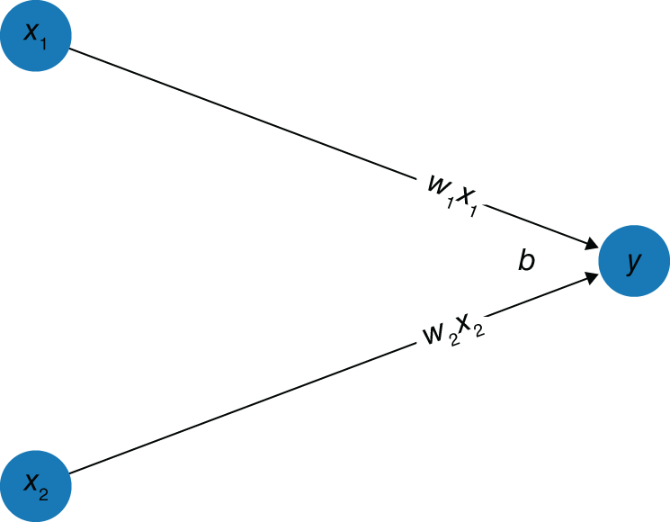
FIGURE 4.6 Visualizing linear regression as a neural network.
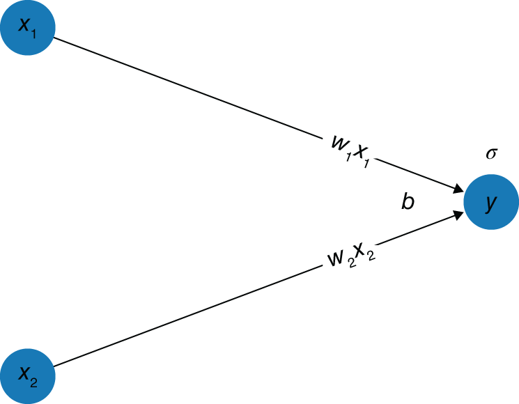
FIGURE 4.7 Visualizing logistic regression as a neural network.
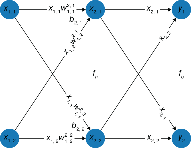
FIGURE 4.8 Visualizing softmax regression as a neural network.
Hopefully, from these examples, we can see that, roughly speaking, a neural network is a system of layers of nodes, each of which feeds forward toward some output, whether that be continuous variables for regression, or class probabilities for classification. It is easy to see how more and more of these layers could be added to move further and further away from the “nice,” “standard” functions we apply to an input and create highly nonlinear, difficult-to-describe relationships between our input and output vectors.
4.2.8.2. Common Types of Neural Networks
Linear, logistic, and softmax regressions are actually all types of feed forward neural network (NN). Although this is one of the most popular types of NN, many others exist. A few popular examples are:
- A feed forward neural network is a type of neural network where connections between the nodes do not form a cycle. In these networks, the information is only passed forward, from the input layer, through the hidden layers (if there are any), and to the output layer. All those shown in the previous sections are types of feed forward neural networks. Feed forward networks are generally further split into two main types:
- A multi-layer perceptron (MLP) is the most standard form of neural network. It consists of an input layer, some number of hidden layers (at least one), and an output layer (see Figure 4.9). Each layer feeds to the next and through an activation function. Specifically, all those shown in the previous sections are MLPs. As shown, they can be used for both regression and classification.
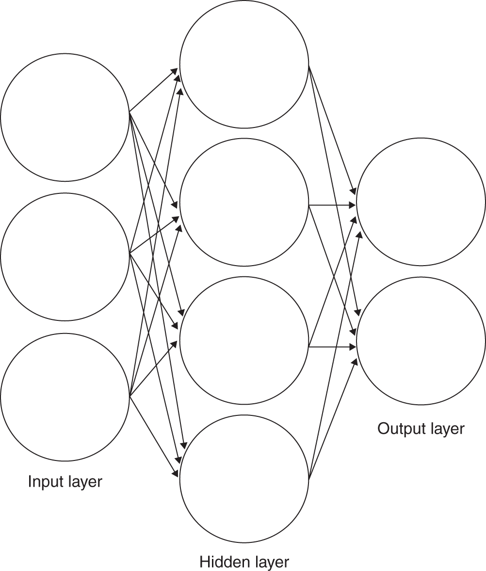
FIGURE 4.9 Multi-layer perceptron with 1 hidden layer.
- Convolutional neural networks (CNNs) are popular for problems where there is some sort of structure between the inputs, such as in an image where adjacent pixels give information about the pixel in question. They are in fact a type of feed forward NN, but typically the 2D/3D structure is kept intact (see Figure 4.10). Generally, one passes some sort of “scanner” or “kernel” over the structure, which takes in some n-by-n(-by-n) subset of the image and applies a function to it, before moving one step right and doing the same. This process is repeated across the image from left to right, top to bottom, until we then have some new layer of transformed images. These layers are built up in a similar way to a standard feed forward NN to eventually yield an output layer. CNNs are particularly good at image detection, both in classifying an image and finding objects within an image. We discuss these in Section 4.5.2, in the context of structuring images.
- A multi-layer perceptron (MLP) is the most standard form of neural network. It consists of an input layer, some number of hidden layers (at least one), and an output layer (see Figure 4.9). Each layer feeds to the next and through an activation function. Specifically, all those shown in the previous sections are MLPs. As shown, they can be used for both regression and classification.
- Recurrent neural networks (RNNs) are a class of artificial neural networks where connections between nodes do not have to point “forward” toward the output, but rather can point in any direction other than back to the input layer. This allows it to exhibit temporal dynamic behavior. Unlike feed forward neural networks, RNNs can use these loops (which act like memory) to process a sequence of inputs. As such, they are useful for tasks such as connected handwriting or speech recognition. Given their temporal nature, the hope is that they could provide a breakthrough in financial time series modeling. LSTMs (long short-term memory) are an extension of RNNs, which enable longer-term dependencies in time to be modeled.
- Autoencoder neural networks are designed for unsupervised learning. They are popularly used as a data compression model to encode input into a smaller dimensional representation, similar to principal component analysis (PCA). They are trained by first converting to this lower-dimensional representation, before then being decoded to reconstruct the inputs back in the original dimensions, with the loss function increasing the more the reconstructed image deviates from the original. We can then take the layers that reduce the dimensionality of our inputs and use this new output (our encoding) as inputs in a separate model.
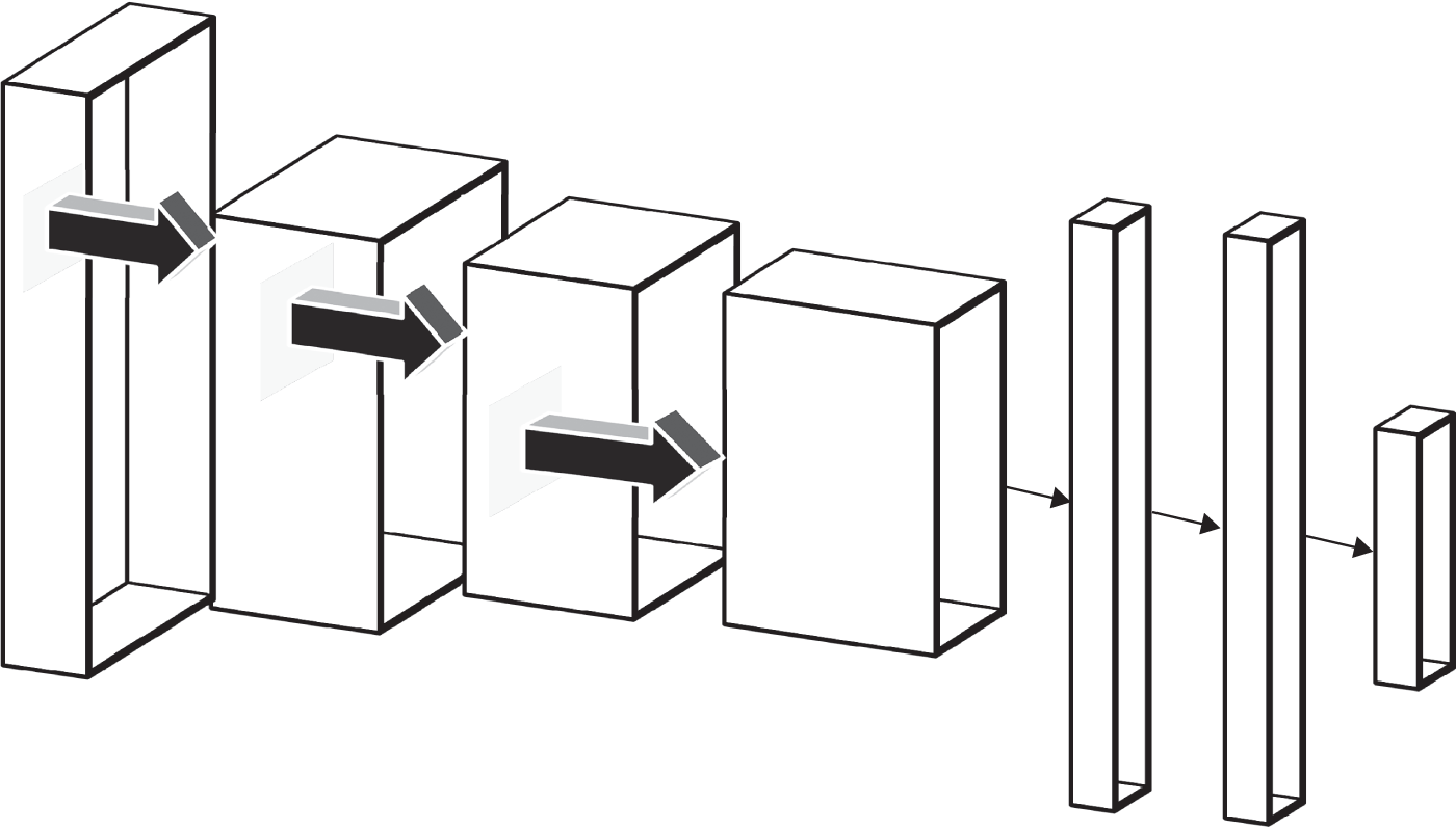
FIGURE 4.10 Convolutional neutral network with 3 convolutional layers and 2 flat layers.
- Generative adversarial neural networks (GANs) consist of any 2 networks working together, typically a CNN and an MLP, where one is tasked to generate content (generative model) and the other to judge content (discriminative model). The discriminative model must decide if the output of the generative model looks natural enough (i.e. is classified as whatever the discriminative model is trained on). The generator attempts to beat the discriminator and vice versa. Through alternating training sessions, one hopes to improve both models until the generated samples are indistinguishable from the real world. GANs are a current hot topic and look as though they could be very useful for image/speech generation. A particular use within finance could be artificial time series generation as discussed by Pardo (2019), as discussed earlier in this chapter when talking about reinforcement learning. Hence, we can create time series that have the characteristics of specific assets (e.g. VIX or S&P 500). Generating these datasets would allow us to create unlimited training data to further develop reinforcement learning–based models.
4.2.8.3. What Is Deep Learning?
Deep learning (DL) involves the use of neural networks having many hidden layers (i.e. “deep” NNs). This depth allows them to represent highly nonlinear functions that pick up on nonobvious relationships within the data. This contrasts to more traditional types of machine learning, where we typically spend a large amount of time doing feature engineering, which relies upon our domain knowledge and understanding of the problem at hand. LeCun, Bengio, and Hinton (2015) give the example of when deep learning has been applied to the problem of image recognition. The problem of image recognition is often cited as being one of the major successes of deep learning. Typically, the first layer will try to pick up edges in specific areas of the image. By contrast, the second layer will focus on patterns made up of edges. The third layer will then identify combinations of motifs that could represent objects. In all these instances, a human hasn't made these features; they are all generated from the learning process.
Due to their large number of parameters, they require a very large training set in order not to overfit. However, it also allows them to be extremely flexible and pick up on highly nonlinear relationships, often resulting in less feature engineering being required, although there might still well be a certain amount of hand tuning involved, such as understanding the number of layers, which we should include in the model.
4.2.8.4. Neutral Network and Deep Learning Libraries
4.2.8.4.1. Low-level deep learning and neutral network libraries Theano and TensorFlow are to NN libraries as NumPy is to SciPy, scikit-learn, and scikit-image. Without NumPy, many popular scientific computing libraries would not exist today and, similarly, without either Theano or TensorFlow, many of the higher-level deep learning libraries popular today would not exist. Below we describe them in more detail and also outline PyTorch.
- Theano. Theano is a Python library used to define, optimize, evaluate, and analyze neural networks. Theano heavily utilizes NumPy while supporting GPUs in a transparent manner. Much like NumPy, although you could build a complete NN using Theano, you probably don't want to, in the same way that you usually don't want to build a logistic regressor from scratch in NumPy, but rather using scikit-learn. Instead, Theano is a library that is often wrapped around by other libraries providing more user-friendly APIs, at the cost of flexibility·
- TensorFlow. Like Theano, TensorFlow is another library that can be utilized to build NNs. Originally developed by Google, it is now open source and extremely popular.
- PyTorch. More recently, PyTorch has been developed as an alternative to Theano and TensorFlow. It uses a vastly different structure to the aforementioned that results in slower performance but is easier to read and, therefore, easier to debug code. PyTorch has become popular for research purposes, whereas Theano and TensorFlow are more popular for production purposes.
Next, we compare these various libraries in more detail.
- PyTorch versus TensorFlow/Theano. So why would one prefer PyTorch over TensorFlow/Theano? The answer is static versus dynamic graphs. We won't get into the nitty-gritty of what static and dynamic graphs are; however, in summary, PyTorch allows you to define and change nodes “as you go,” whereas in TensorFlow and Theano, everything must be set up first and then run. This gives PyTorch more flexibility and makes it easier to debug but also makes it slower. Furthermore, some types of NN benefit from the dynamic structure. Take an RNN used for natural language processing (NLP). With a static graph, the input sequence length must stay constant. This means you would have to set some theoretical upper bound on sentence length and pad shorter sentences with 0s. With dynamic graphs, we can allow the number of input nodes to vary as is appropriate.
- Theano versus TensorFlow. If one has decided on Theano or TensorFlow over PyTorch, the next decision is, therefore, Theano or TensorFlow. When deciding between the two, it is important to consider a few things:
- Theano is faster than TensorFlow on a single GPU, whereas TensorFlow is better for multiple GPUs/distributed systems, as many of those in production are today.
- Theano is slightly more verbose, giving more finely grained control at the expense of coding speed.
- Most importantly, however, the Montreal Institute for Learning Algorithms (MILA) have announced that they have stopped developing Theano since the 1.0 release. Indeed since 2017, there have only been very minor releases.
- As such, the general consensus seems to be that people prefer TensorFlow, with TensorFlow having 41,536 users, 8,585 watchers, and 129,272 stars on GitHub to Theano's 5,659, 591, and 8,814 respectively at time of print.
It is somewhat a case of “horses for courses,” however. TensorFlow is likely the safer bet if one must decide between the two. Another consideration when it comes to performance is the cloud environment one is using.
4.2.8.4.2. High-level deep learning and neutral network libraries For many purposes, users might prefer higher-level libraries to interact with neural networks, which strip away some of the complexity of dealing with low-level libraries like TensorFlow.
- Keras. As previously mentioned, there exist many equivalents to scikit-learn, but for NNs, the most popular of which is probably Keras. Keras provides a high-level API to either TensorFlow or Theano; however, Keras is optimized for use with Theano. Google have integrated Keras into TensorFlow from version 2 onwards.
- TF Learn. Like Keras, TF Learn is a high-level API, however, this time optimized for TensorFlow. Strangely, although TF Learn was developed with TensorFlow in mind, it is Keras that seems to be more popular on GitHub with 27,387 users, 2,031 watchers, and 41,877 stars to TF Learn's 1,500, 489, 9,121 respectively at the time of writing. In that sense, it is not as clear which of the two to use between Keras or TF Learn as it is with Theano and TensorFlow.
4.2.8.4.3. Middle level deep learning and neutral network libraries
- Lasagne. Lasagne is a lightweight library used to construct and train networks in Theano, being less heavily wrapped around Theano than Keras is, providing fewer restraints at the cost of more verbose code. Lasagne acts as a middle ground between Theano and Keras.
4.2.8.4.4. Other frameworks While TensorFlow has become one of the most dominant libraries for neural networks and has become a core part of many higher-level libraries, it is worth noting that there are frameworks available, some of which we discuss here.
- (Apache) MXNet. Although it offers a Python API, MXNet is technically a framework rather than a library. The reason we discuss it is that, although it does have a Python API, it also supports many other languages, including C++, R, Matlab, and JavaScript. Furthermore, MXNet is developed by Amazon and, as such, was built with AWS in mind. Although MXNet takes a bit more code to set up, it is well worth it if you plan to perform a large amount of distributed computing using, say, AWS, Azure, or YARN clusters. Finally, MXNet offers both an imperative programming (dynamic graph) structure, like PyTorch, and a declarative programming (static graph) structure, like Theano and TensorFlow.
- Caffe. Unlike the other frameworks previously mentioned, Caffe does not provide a Python API in the same way that the others do. Instead, you define your model architecture and solver methods in JSON-like files called .prototxt configuration files. The Caffe binaries use these .prototxt files as input and train your network. Once trained, you can classify new images using the Caffe binaries or through a Python API. The benefit of this is speed. Caffe is implemented in pure C++ and CUDA, allowing roughly 60 million images per day to be processed on a K40 GPU; however, it can make training and using models cumbersome, with programmatic hyperparameter tuning being particularly difficult.
4.2.8.4.5. Processing libraries Another thing to consider when using alternative data is preparing your data. Although data vendors may provide you with the raw data you require, it may not be labeled or processed for you. Here we focus on general-purpose libraries. Later, in the book, we also discuss libraries specifically relevant for common tasks in structuring alternative data, namely image processing and natural language processing.
- NumPy. Although you probably know about NumPy already, many do not utilize it to its full extent. NumPy can be particularly useful when utilized properly due to its vectorized functions. Want to create an image mask? If your image is loaded into a numpy.ndarray, simply type
mask = image < 87. Want to set pixels under that mask to white?image[mask] = 255. Although rudimentary, NumPy is very powerful and should not be overlooked. - Pandas. Similar to NumPy, Pandas has an enormous arsenal of useful (vectorized) functions for us to use, making data preprocessing far easier than with standard Python alone.
- SciPy. What can be thought of as an extension of NumPy, SciPy offers another vast set of useful preprocessing functions. From splines to Fourier transforms, if there is some special mathematical/physical function you desire, SciPy is the first place you should look.
4.2.9. Gaussian Processes
In this section, we hint at another useful technique that has come to the fore recently – Gaussian processes (GP). GPs are general statistical models for nonlinear regression and classification that have recently received wide attention in the machine learning community. Given that any prediction is probabilistic when we use Gaussian processes, we can construct confidence intervals to understand how good the fit is. Murphy (2012) notes that having this probabilistic output is useful for certain applications, which include online tracking of vision and robotics. It is also reasonable to conclude that such probabilistic information is likely to be useful when it comes to making financial forecasts.
Gaussian processes were originally introduced in geostatistics (where they are known under the name “Kriging”). They can be also used to combine heterogeneous data sources, which occurs frequently in alternative (and non-alternative) data applications. Work has been done in this area by Ghosal et al. (2016), who use GPs to combine the following data sources: technical indicators, sentiment, option prices, and broker recommendations to predict the return on the S&P 500. Before discussing the paper of Ghosal (2016), we will briefly illustrate Gaussian processes based on that paper. For more details we refer the reader to Rasmussen (2003).
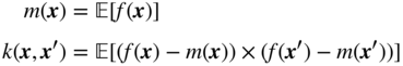
A Gaussian process is a collection of random variables, any finite subset of which has a joint Gaussian distribution. Gaussian processes are fully parametrized by a mean function and covariance function, or kernel. Given a real process, ![]() , a Gaussian process is written as:
, a Gaussian process is written as:
with ![]() and
and ![]() respectively the mean and covariance functions:
respectively the mean and covariance functions:
with centered input set ![]() , output set
, output set ![]() . The Gaussian Process
. The Gaussian Process ![]() , the distribution of
, the distribution of ![]() is a multivariate Gaussian:
is a multivariate Gaussian:
where ![]() . Conditional on
. Conditional on ![]() , we have:
, we have:
where ![]() parameterizes the noise. Due to the Gaussian distribution being self-conjugate, we have the following marginalization (independent of
parameterizes the noise. Due to the Gaussian distribution being self-conjugate, we have the following marginalization (independent of ![]() , i.e. for a point in general, possibly where we have no observations):
, i.e. for a point in general, possibly where we have no observations):
When it comes to making a prediction, ![]() , at some new unseen point,
, at some new unseen point, ![]() (i.e. conditioning on the training data) we then have that:
(i.e. conditioning on the training data) we then have that:
where ![]() ,
, ![]() and
and ![]() .
.
This setup allows us to encode prior knowledge of ![]() through the covariance function
through the covariance function ![]() with observation data to create a posterior distribution based on our observations. The choice of
with observation data to create a posterior distribution based on our observations. The choice of ![]() , often called a kernel, allows us to dictate what behavior we would expect from points based on their proximity to one another. One such as the Gaussian Radial Basis Function allows us to encode the fact that points nearby in vector space should realize similar values of
, often called a kernel, allows us to dictate what behavior we would expect from points based on their proximity to one another. One such as the Gaussian Radial Basis Function allows us to encode the fact that points nearby in vector space should realize similar values of ![]() .
.
As Chapados (2007) points out, Gaussian processes differ from neural networks in that they rely on a full Bayesian treatment, providing a complete posterior distribution of forecasts. In the case of regression, they are also computationally relatively simple to implement. In fact, the basic model requires only solving a system of linear equations, albeit one of size equal to the number of training examples, that is, requiring ![]() computation. However, one of the drawbacks of Gaussian processes is that they tend to be less well suited to higher-dimensional spaces.
computation. However, one of the drawbacks of Gaussian processes is that they tend to be less well suited to higher-dimensional spaces.
As explained by Chapados (2007), a problem with more traditional linear and nonlinear models is that making a forecast at multiple time horizons is done through iteration in a multi-step fashion. Furthermore, conditioning information, in the form of macroeconomic variables, can be of importance, but exhibits the cumbersome property of being released periodically, with explanatory power that varies across the forecasting horizon. In other words, when making a very long-horizon forecast, the model should not incorporate conditioning information in the same way as when making a short- or medium-term forecast. A possible solution to this problem is to have multiple models for forecasting each time series, one for each time scale. However, this is hard to work because it requires a high degree of skill on the part of the modeler, and is not amenable to robust automation when one wants to process hundreds of time series. Chapados (2007) offers a GP-based solution to forecasting the complete future trajectory of futures contracts spreads arising on the commodities markets.
As for Ghoshal (2016), they analyze 12 factors that are thought to be signals for the next day's S&P 500 returns, split into technical, sentiment, price-space, and broker-data groups. They choose those deemed to have a significant correlation with the target to analyze further, namely; (1) 50-day SMA; (2) 12-day, 26-day, exponential MACD; (3) Stocktwits sentiment factor; (4) a “directionality” factor and; (5) a “viscosity” factor. Testing both stationary and adaptive Gaussian process models, they show that they can outperform their stationary/adaptive autoregressive model benchmarks in both cases, even when just using factors from one group. Furthermore, they also show how GP models can give us the relevance of a factor (either stationary over a whole period or adaptive over time). We will present an application of GPs in the case study in Chapter 10.
4.3. WHICH TECHNIQUE TO CHOOSE?
There is no general-purpose algorithm that can provide a best solution for all the problems at hand. Every problem, depending on its domain, complexity, accuracy, and speed requirements, might warrant a different methodological approach, and hence will result in different best-performing algorithms. The no-free-lunch (NFL) theorems have been stated and proven in various settings11 centered on supervised learning and search. They show that no algorithm performs better than any other when their performance is averaged uniformly over all possible problems of a particular type. This means that we need to develop different models and different training algorithms for each of them to cover the diversity of problems and constraints we encounter in the real world.
With the mass advent of unstructured data, we may need to use more advanced techniques to those traditionally used within finance. For example, the analysis of unstructured data such as images cannot yield good results with the standard statistical tools. Logistic regression can be used for this task, but the classification accuracy is generally low. There have been recent developments in the machine learning field that now allow us to analyze images, text, and speech with a higher level of accuracy. Deep learning is one such development. Deep learning for a variety of image recognition tasks, for example, has surpassed human performance.12 We discussed deep learning in Section 4.2.8.
We itemize the techniques typically used to solve the most common types of problems, based on our experience (see Table 4.1). The list is not exhaustive and techniques different from the ones in the list could also fare well, so the reader should take this list as a starting map, not an absolute prescription. We will describe typical use cases that are of interest to the financial practitioner in the left column of the table. Corresponding suggestions are in the right column, many of which use models we have discussed earlier in this chapter. We also refer the reader to Kolanovic and Krishnamachari (2017), which has a larger list of various finance-based problems and potential machine learning methods that can be used to solve them.
TABLE 4.1 Financial (and non-) problems and suggested modeling techniques.
| Market regime identification | Hidden Markov Model |
| Future price direction of assets, basket of assets and factors | Linear regression, LSTM13 |
| Future magnitude of price change of assets, basket of assets and factors | Linear regression, LSTM |
| Future volatility of assets, basket of assets and factors | GARCH (and variants), LSTM |
| Assets and factors clustering and how it changes over time | K-means clustering, SVM |
| Asset mispriced to the market | Linear regression, LSTM |
| Probability of an event occurring (e.g. market crash) | Random forests |
| Forecast company and economic fundamentals | Linear regression, LSTM |
| Forecast volume and flow of traded assets | GARCH (and variants), LSTM |
| Understanding market drivers | PCA |
| Events study (reaction of prices to specific events) | Linear regression |
| Mixing of multi-frequency time series | Gaussian processes |
| Forecasting changes in liquidity of trading | Linear regression, LSTM |
| Feature importance in asset price movements | Random forest |
| Structuring | |
|
Convolutional neural networks |
|
BERT,14 XLNet15 |
|
Deep neural networks–Hidden Markov model |
|
Convolutional neural networks |
| Missing data imputation | Multiple singular spectral analysis |
| Entity matching | Deep neural networks |
In the latter part of this chapter we give some practical examples of using various techniques for structuring images and text.
In order to select the best method to analyze data, it is necessary to be acquainted with different machine learning approaches, their pros and cons, and the specifics of applying these models to the financial domain. In addition to knowledge of models that are available, successful application requires a strong understanding of the underlying data that are being modeled, as well as strong market intuition.
4.4. ASSUMPTIONS AND LIMITATIONS OF THE MACHINE LEARNING TECHNIQUES
Machine learning and, in general, quantitative modeling is based on assumptions and choices made at the modeling stage whose consequences we must be aware of. They seem trivial but in practice we have seen a lack of awareness about what these assumptions entail. First, there is difference between causality and correlation and it is the former we need most of the time when making predictions. Second, nonstationary data makes learning very difficult and unstable in time, yielding unreliable results. Third, it is important to bear in mind that a dataset we work on is always a subset of variables that might drive a phenomenon. Precious information that can complement a dataset might lie in other, different datasets, or even in our expert knowledge. Last, the choice of the algorithm must be determined given its known limitations, the data at hand, and the business case. We now turn to discuss these aspects in detail.
4.4.1. Causality
In the previous sections, we have provided a list of suggested different machine learning techniques according to the use case but there is a common aspect (and a potential problem) to many of the applications that we must be aware of. In classification (prediction) tasks we always try to learn the functional relationship between a set of inputs and an output(s). In doing so, we will likely encounter an old known problem – spurious correlations, or statistical coincidences. But even if a relationship between two variables is causal (i.e. there is no third variable acting as a confounder), a neural network, or even the much simpler linear regression, cannot tell the direction of causality, and hence input and output can be exchanged finding equally strong association.
Nevertheless, for certain tasks, in order to have a robust model, one that does not frequently need recalibration and whose results hold through time, solid domain-specific reasoning is warranted when building it.16 This is to say that the causes must be the inputs to a model trying to predict an output (the effect). As Pearl (2009) points out, causal models have a set of desirable characteristics. To use his terminology, casting a treatment of a problem in terms of causation:
- Will make the judgments about the results “robust”
- Will make them well suited to represent and respond to changes in the external environment
- Will allow the use of conceptual tools that are more “stable” than probabilities
- Will also permit extrapolation to situations or combinations of events that have not occurred in history
When it comes to practicalities one must make sure that the processes by which the training data is generated are stable and that the relationships being identified are relationships that occur because of these stable causal processes. This can be a tricky task as most of the time causal relationships between variables are not known or nonexistent. However, we must be sure that we have inputted the best of our domain knowledge into the problem at hand. This leads us to another important point: stationarity.
4.4.2. Non-stationarity
The lack of stationarity is very tricky to deal with and in most cases machine learning models cannot cope with it. In fact, learning always assumes that the underlying probability distribution of the data from which inference is made stays the same. This is a condition that is hardly encountered in practice. We note that stationarity does not ensure good (or any) predictive power as it is a necessary but nonsufficient condition for the high performance of an algorithm. If we take the examples where deep learning has been particularly successful, it has typically been where the characteristics of the underlying dataset are relatively static, such as identifying cats in photos17 or counting cars in parking lots or language translation.
The change in the distribution of data contained in development/test datasets versus the data in the real world on which a model is subsequently applied is called dataset shift (or drifting). Dataset shift could be divided into three types: (1) shift in the independent variables (covariate shift), (2) shift in the target variable (prior probability shift), and (3) shift in the relationship between the independent and the target variable (concept shift). Only the first type has been extensively studied in the literature (see e.g. Sugiyama, 2012) and there are some recipes of dealing with it while the other two are still being actively researched.
Financial time series exhibit non-stationarity, such that properties like their mean and variance can change significantly and the underlying probability distribution can change in a totally unpredictable way. This can be particularly observed during periods of market turbulence where there are structural breaks in the time series of many variables (e.g. volatility). These can be especially brutal for, say, managed currencies, where volatility is kept artificially low through central bank intervention and then explodes when central banks no longer have sufficient funds to keep the currency within a tight bound.
4.4.3. Restricted Information Set
Another important point is that any algorithm is trained on a restricted information set – both number of features and history – given by the specific dataset. Thus the insights that can be derived are inherently limited to what is contained in that dataset. In this sense, algorithms are blind to what happens outside of their narrow world. Essentially, data you have does not tell you about the data you do not have. To borrow the terminology popularized by Donald Rumsfeld, these are essentially known unknowns.
This could become quite problematic when trying to predict market crashes, which are rare events. Often early warning indicators can be found by looking outside the dataset and be integrated with the findings of an algorithm that operates on that dataset. However, the triggers for market crashes can vary significantly. For example, indicators within the emerging markets may have been useful for predicting many crises in the early 2000s and in particular the Asian Crisis in 1997. However, they would not have been as important for predicting the global financial crisis, which emanated from developed markets, such as in US subprime, before spreading. Variables related to developed market credit spreads would have been far more insightful in this instance than those related to emerging markets that moved later after the contagion. Commonly this can be done through a human-in-the-loop intervention to correct or complement the inputs/outputs of a model. In this case humans can exceed algorithms as knowledge of the context is sometimes more useful than tons of past data. Humans are sometimes extremely good at prediction with little data. We can recognize a face after seeing it only once or twice, even if we see it from a different angle or years after we last saw it. Deep learning algorithms, on the other hand, require hundreds if not thousands of images in the training set.
See Agrawal et al. (2018) for a more detailed reasoning on this topic. Of course, there are also the unknown unknowns. These elude both machines and humans. Last, in Agrawal et al.'s lingo (but not in Rumsfeld's), there are the unknown knowns where the algorithm gives an answer with a great confidence, but this can be spurious because the true underlying causality is not understood by it. We refer to Agrawal et al. for more details.
4.4.4. The Algorithm Choice
Finally, the choice of an algorithm – another assumption – will be important in the use case at hand and it must be guided by the nature of the problem we are trying to solve and the amount of data available. As already mentioned, there is no best-performing universal algorithm. Deep learning models do an excellent job counting cars in parking lots, or extracting sentiment from text, but they might not perform as well when predicting financial time series, in particular for lower-frequency data. Where data is particularly scarce, we could find that simpler machine learning techniques such as linear regression may be a better choice than more complicated deep learning approaches.
So what are the typical problems we face in finance? First, financial time series have a low signal-to-noise ratio. Image recognition systems are very sensitive to noise. Hence, for instance, adding some white noise to an image could completely alter the result of a classification. Second, the amount of data is sometimes not sufficient because deep learning is known to be data greedy. We can enlarge the sample to include more data points from the past. However, we may encounter the non-stationarity issues discussed in Section 4.4.2 given the continually changing nature of markets and the economy. For example, this approach is unlikely to be useful to backtest a high-frequency trading strategy, if we end up examining historical periods when the market was dominated by human market makers and had a very different market microstructure. These types of markets were very different from subsequent periods when electronic traders have come to dominate short-term price action.
We could use deep learning techniques, such as LSTM (long short-term memory) to explore time series from high-frequency order book data. As we noted earlier in this chapter, the benefit of LSTM over ordinary recurrent neural networks (RNNs) is that they can capture longer-term dependencies in the data while also forgetting less relevant events. Hence, LSTMs can learn over many time steps. The ability to be able to explain these longer-term dependencies is key to time series modeling. Indeed, without the ability to model longer term relationships in a time series, we would have difficulty modeling many patterns. These patterns would, for example, include those associated with seasonality (for example, time of day, day of the week, etc.).
In a high-frequency trading environment, we have very large amounts of data to train such a model, not only the number of trades executed but also the much larger dataset of all published quotes. Even in this instance, there are still likely to be multiple challenges, in particular making sure that once a model is trained, it can be executed quickly. If a high-frequency trading model cannot be run sufficiently quickly, then it will be impossible to monetize any of its trade recommendations. High-frequency trading strategies are often very latency sensitive.
Bearing all these issues in mind for the future, we now turn to discussing image and text structuring and understanding.
4.5. STRUCTURING IMAGES
4.5.1. Features and Feature Detection Algorithms
When interpreting an image, humans try to focus on important elements and often ignore much of the image. In a sense, we are subconsciously doing a dimensionality reduction of the data. The principle is similar in computer vision where we might seek to convert an image into a feature vector. Many alternative datasets that are relevant for finance are originally derived from images. While it might be possible for a human to interpret an image, when the volume of images becomes significant, this is not possible. Hence, having effective automated techniques to process these images is important. In Chapter 13, we specifically give use cases for satellite imagery for investors. These datasets can be derived from many thousands of images that would be very costly to process in a manual way and would also be prone to inconsistencies.
In image recognition, we essentially seek to extract important features from an image, which we hope are most useful for understanding its content. Salahat and Qasaimeh (2017) discuss some ideal properties of such features, which we summarize here. Some features within the image can be related to boundaries. Edges occur where there are sudden changes in the pixel intensity. Corners, meanwhile, occur where edges join. Some features are based on blobs or regions. Different blobs will be differentiated by differences in terms of brightness, color, and so on. Figure 4.11 presents a summary of various feature detector algorithms, breaking them down by their category and what their classifier is based on (Salahat and Qasaimeh, 2017).
So what are the ideal properties of features? Features should be distinctive so they can be distinguished from one another. They need to cover a relatively small area. In other words, they need to be local. It needs to be computationally efficient to compute the features. This is particularly relevant if we are using them for real-time applications, such as detecting objects in real-time video feeds.
Features should be repeatable, so should be relatively stable from frame to frame. For this to be the case, they need to be invariant to changes in perspective and rotation. A horse, for example, looks very different in profile compared to head on. Regardless of the angle of its image, it is still very much a horse. Furthermore, they shouldn't be affected by factors impacting image quality such as noise, blur, and compression artifacts. In Figure 4.12, we list some of the various feature detector algorithms and how they fare in terms of these various idealized feature qualities from Salahat and Qasaimeh (2017).
| Category | Classification | Methods and Algorithms |
| Edge-based | Differentiation based | Sobel, Canny |
| Corner-based | Gradient based | Harris (and its derivatives), KLT, Shi-Tomasi, LOCOCO, S-LOCOCO |
| Corner-based | Template based | FAST, AGAST, BRIEF, SUSAN, FAST-ER |
| Corner-based | Contour based | ANDD, DoG-curve, ACJ, Hyperbola fitting, etc. |
| Corner-based | Learning based | NMX, BEL, Pb, MS-Pb, gPb, SCG, SE,tPb, DSC, Sketch Tokens, etc. |
| Blob (interest point) | PDE based | SIFT (and its derivatives), SURF (and its derivatives), CenSurE, LoG, DoG, DoH, Hessian (and its derivatives), RLOG, MO-GP, DART, KAZE, A-KAZE, WADE, etc. |
| Blob (key point) | Template based | ORB, BRISK, FREAK |
| Blob (interest region) | Segmentation based | MSER (and its derivatives), IBR, Salient Regions, EBR, Beta-Stable, MFD, FLOG, BPLR |
Source: Based on data from Salahat and Qasaimeh (2017).
FIGURE 4.11 Various edge, corner, and blob-based feature detectors.
| Features Detector | Rotation | Invariance Scale | Affine | Repeatability | Qualities Localization Robustness | Robustness | Efficiency |
| Harris | Y | – | – | +++ | +++ | +++ | ++ |
| Hessian | Y | – | – | +++ | ++ | ++ | + |
| SUSAN | Y | – | – | ++ | ++ | ++ | +++ |
| Harris-Laplace | Y | Y | – | +++ | +++ | ++ | + |
| Hessian-Laplace | Y | Y | – | +++ | +++ | +++ | + |
| DoG | Y | Y | – | ++ | ++ | ++ | ++ |
| Salient Regions | Y | Y | Y | ++ | + | ++ | + |
| SURF | Y | Y | – | ++ | +++ | ++ | +++ |
| SIFT | Y | Y | – | ++ | +++ | +++ | ++ |
| MSER | Y | Y | Y | +++ | +++ | ++ | +++ |
Source: Based on data from Salahat & Qasaimeh (2017).
FIGURE 4.12 Dominant feature detection algorithms and their properties.
So how can we use these features in practice for a computer vision problem like image classification? The first step is to label the images we have, for example, “burger” and “other.” Then we need to convert all the images into their respective feature vector representations by using a feature detector algorithm. The problem can then be solved as a classification-style supervised machine learning problem. In this instance, we are essentially trying to partition a high-dimensional hyperspace into areas for “burger” and “other.” Our hyperspace consists of many points, each of which feature a vector representing an image. We could attempt to use a linear model, such as logistic regression to partition this space. However, it is likely that nonlinear techniques like SVMs (support vector machines) would yield better results.
4.5.2. Deep Learning and CNNs for Image Classification
Our discussion on computer vision has largely centered on constructing feature vector representations using feature detection algorithms related to edges, corners, and blobs. This approach seems intuitive given its similarity to the way we interpret an image. Is there a better way to extract features that could yield better accuracy for example for image recognition? Potentially can we automatically identify higher-level features? Would this do a better job than a feature detection algorithm where we preprocess an image for features based on intuitive features like corners?
We can use deep learning to “discover” appropriate features, as mentioned earlier in this chapter, as opposed to trying to create them ourselves by hand (i.e. feature engineering). In particular, convolutional neural networks have been successful in the area of image recognition, as we mentioned earlier. A CNN essentially skips the step where we apply a feature detection algorithm. Instead, it uses raw pixel data as an input feature map, where each pixel is basically a vector consisting of entries of red, green, and blue values. We can think of the convolution operation as a sliding tile, which sweeps over the original image. As the tile slides over the image on overlapping parts of the image, it creates an output feature map, constructing a dot product. In other words, it does a summation over the elementwise multiplications with a set of weights. The size of the “slide” is known as the stride. Dumoulin and Visin (2018) explains the impact of the stride and other factors in the convolution operation.
This matrix of weights is known as a filter. Traditionally, the filter would have been handcrafted to pick up specific relatively intuitive features, such as a horizontal, vertical, or diagonal edge. However, in this case, we instead start with randomized weights, which are later “fitted,” so we can learn the important features, rather than prespecifying them.
It is common to have multiple filters applied, which increases the depth of the output. It is important to note that the convolution step allows us to keep some of the relationship between pixels that are near to each other. If this relationship was lost, it would make it much more difficult to make sense of the image. The more filters are used, the more features can be extracted by the CNN.
A nonlinearity is then introduced to the convoluted feature using a Rectified Linear Unit (ReLU). The ReLU outputs the maximum of each matrix element and zero. Recalling our introduction to neural networks, this is a prominent recent example of an activation function. Following this, there is the pooling step, where the convolution feature is downsampled. This reduces the number of parameters and hence reduces computation time necessary when training the network. There can be several convolutional and pooled layers after each other. The idea is that through these multiple steps we can capture the important parts of the image for classification purposes while discarding the less relevant parts.
After the convolutional and pooled layers, we flatten the image into a long vector. The next step is to have some fully connected layers, which perform the classification step for the ![]() classes of objects we wish to identify. The final connected output layer will give a probability for the input image matching a classification such as “Is this a burger?” The network can be trained to fit the optimal weights through backpropagation. Typically, techniques based upon CNN are far more prevalent these days when it comes to image classification, compared to those using handcrafted features. The downside of such techniques is that it can sometimes be more difficult to understand why a certain output has been generated, because the features created may not always be intuitive. We could argue that for image recognition this is less of a concern, because the task they are performing is simply automating a task that a human can do and check.
classes of objects we wish to identify. The final connected output layer will give a probability for the input image matching a classification such as “Is this a burger?” The network can be trained to fit the optimal weights through backpropagation. Typically, techniques based upon CNN are far more prevalent these days when it comes to image classification, compared to those using handcrafted features. The downside of such techniques is that it can sometimes be more difficult to understand why a certain output has been generated, because the features created may not always be intuitive. We could argue that for image recognition this is less of a concern, because the task they are performing is simply automating a task that a human can do and check.
4.5.3. Augmenting Satellite Image Data with Other Datasets
Recognizing objects from a satellite image can be done using the techniques described earlier. However, this is not the only step we need to structure image data in order for it to be useful for investing purposes. For each satellite image, there is associated geospatial data, such as GPS coordinates, the timestamp, and so on. This data can be joined with datasets containing addresses. As a result, the objects detected on the image can be annotated with additional tags. These tags can help us answer questions we can't answer from the satellite image alone. These questions can include whether the location is associated with a particular business, which particular city and country it is in, and so on. Typically, we might also wish to understand changes in a location over time, in particular if we wish to construct time series for use by investors. We give a use case later in the book in Chapter 13, where we discuss how investors can use satellite imagery of retailer car parks to help forecast earnings per share for these companies.
4.5.4. Imaging Tools
In practice, if we want to process images, there are many existing libraries that can help us, including:
- scikit-image. Another member of the scikit family, scikit-learn, while not offering anything particularly fancy, offers a clean and simple API that is quick to pick up with a plethora of useful functions. Want to find edges with a Sobel filter?
edges = skimage.filters.sobel(image). - SciPy.ndimage. Probably one of SciPy's lesser known submodules is scipy.ndimage. Providing many functions that can be applied to numpy.ndarrays it certainly comes in handy now and then. Want to blur an image?
scipy.ndimage.gaussian_filter(image, sigma=1). - Matplotlib. Although generally used in analysis/exploration, matplotlib offers a GUI to interact with images and can be used for centroid/bounding-box labeling by using its event handling capabilities.
- Pillow. Pillow, a fork from the now deprecated PIL, offers many basic image processing functions, such as brightness and contrast altering functions.
- OpenCV. Open CV is another framework that offers a Python API. A very powerful library with many pre-trained models, one could spend a lifetime learning all the ins and outs of OpenCV.
- SimpleCV. SimpleCV can be thought of as the Keras of image processing. It offers access to several computer vision libraries, such as OpenCV, but with a higher-level wrapper, resulting in a shallower learning curve.
4.6. NATURAL LANGUAGE PROCESSING (NLP)
4.6.1. What Is Natural Language Processing (NLP)?
Many alternative datasets consist of text. The web itself consists mostly of text. If we ignore text-based data on the web, we are essentially ignoring a lot of information that could potentially be useful from an investment perspective. In Chapter 15, we discuss many investment use cases for text, ranging from using social media to help make economic data estimates to using news sentiment to understand market sentiment. In order to make trading decisions using text data, we have to go through a number of steps. In particular, given the volume of text data, we need to have automated ways to analyze text. This is where natural language processing (NLP) can help us.
In a nutshell, NLP can be seen as a way for a computer to understand human language. However, in order to do NLP, we should first define the various parts of natural language. Briscoe (2013) describes the various components of natural or human language and gives an overview of NLP.
At the lowest level we have phonetics, which involves the specific sounds generated by a human. Built on top of this we have phonology, which examines the sounds of a particular language. The next level, morphology, looks at how words have been constructed and their decomposition. For example, the word “burgers” can be broken down into “burger” (which is a root) and “s” (which is a suffix showing plurality). We can have many other types of construction, such as different verbal forms like eating (verb), eating (adjective), and eating (noun). For certain languages, such as Arabic, morphology can be very important. At their root, Arabic verbs usually consist of three root letters (or sometimes four letters in certain cases) from which we can derive many different verb forms and related words, such as verbal nouns, which in other languages may have different roots. For example, in Arabic the verbs for “to teach” and “to learn,” which have related meanings, have the same root. This contrasts with English where each word is totally different.
Syntax is the way in which words are combined to make sentences. The grammar will dictate how words can be combined together to form a grammatically correct sentence. Some languages, such as English, have the word order SVO (subject-verb-object). By contrast, Arabic tends to be VSO (verb-subject-object). However, for any particular set of words, there are likely to be several different grammatically correct word orders, each of which have different meanings. For example, both “Alex consumes burgers” and “Burgers consume Alex” are grammatically correct, but clearly they have totally different meanings. Indeed, in English, without any word order there would likely be a significant amount of ambiguity for the meanings of words. Potentially, though, we could have a more flexible ordering where words change depending on their place in a sentence, which is referred to as an inflected language. Latin is an example of such a language, where extensive use of case endings lets us tell whether, for example, a word is a subject or an object, without the need to adhere to a strict word order.
Semantics is about the meaning of language. We should be able to understand a sentence so we can answer questions like who, what, why, where, how, and when. Pragmatics refers to understanding the text with context, which often requires knowledge of information beyond the text itself.
NLP attempts to tackle problems at the various levels described above. Doing any sort of analysis of syntax first involves word tokenization/segmentation to identify words. We can then do other NLP tasks such as tagging the parts of speech (e.g. that words are nouns, verbs, adverbs, and so on).
At the semantic level, there are also a number of important NLP tasks. One of the most important is named entity recognition, to identify specific people, organizations, locations, and so on, and also being able to do relation extraction between their entities. An ability to extract the events and the temporal meaning is key. This is particularly true from the context of an investor, where we are likely to place more weight on forward-looking statements, compared to a review of historical market moves.
We also need to identify the semantic roles in the sentence, such as identifying the agent of the action and the target. More simply, an example of this can be asking, “Who is doing what to whom?” Again, this is very important for understanding the significance of a statement. If the president of the United States calls for sanctions against an oil-producing nation, this is of more relevance than a State Department spokesperson. Semantic role labeling is an automatic way to find these roles. We also have sentiment analysis to understand how positive or negative a text is. We might also wish to do topic recognition to identify the general subjects being discussed in a document.
NLP can therefore help us in our task of adding metadata to a particular text helping to identify the following:
- Topic of the content: What is it generally about politics, economy, the weather, and so on?
- Entities listed in the content: Are there any specific people mentioned, or companies, and in particular do they relate to any tradable assets?
- Sentiment of the content: Is it broadly positive or negative?
In the following sections, we briefly examine a few topics from NLP. For readers wishing to have an in-depth and more exhaustive look at NLP, we recommend reading Jurafsky and Martin (2019) and we have used that as a reference in this chapter. There are also many other tasks in NLP that are not related to understanding only. They can involve generation and summarization of text, too.
4.6.2. Normalization
Normalization involves breaking down the text into a more common form. Word segmentation or tokenization involves identifying separate words in text. In English, words are generally broken up by spaces, but we need to be aware of many exceptions. For example, “Burger King” could be considered a word despite having a space. At the same time, we also need to be aware of words that might be written in different ways, such as “KFC” instead of “Kentucky Fried Chicken,” which are specific named entities. Other languages such as Chinese need different techniques for word tokenization. Jurafsky and Martin (2019) discuss using a maximum matching algorithm for word tokenization for Chinese, which requires a dictionary of Chinese. By contrast this algorithm has more difficulties in English. Sentence segmentation, as the name suggests, involves identifying separate sentences. Again, we might be able to utilize full stops as a marker, but need to be careful so we are not confused by full stops used in other contexts like initials. Once the words have been separated, we can put the words into more common forms, which involves lemmatization and stemming. The words “ate,” “eaten,” and “eats” are just different forms of the same verb. Lemmatization would involve normalizing them to the root form “eat.” Stemming involves the simpler normalization of words like rendering plural nouns into their singular form. Obviously, what constitutes a word depends on the language!
A large number of common words are also unlikely to help with understanding the text and are simply used for grammatical reasons, such as “the” and “a.” These are classified as stop words and are typically removed during the normalization stage. However, as in our previous example of “Burger King,” we need to be wary of removing stop words, which could cause issues with named entity recognition. Let's take the example of the pop band “The 1975.” We could use it in that specific context – for example, “The 1975 won a Brit award.” However, another obvious context would be using it to refer to something that occurred in the year 1975, such as “The 1975 United Kingdom European Communities membership referendum resulted in entry to Europe.” If we had removed the stop word of “The,” it would have caused issues of understanding for the first sentence but not for the second sentence.
4.6.3. Creating Word Embeddings: Bag-of-Words
One of the simplest techniques to analyze a text involves using a technique known as bag-of-words. This ignores concepts like word order or grammar. Here we represent the words as a “bag,” which consists of words and their associated frequency in the text. This is essentially a type of vectorized representation of our text, which is called word embedding.
There are many other ways to create word embeddings aside from bag-of-words. TF-IDF can also be used, which weights the importance of words. Another approach is to use n-grams. Here we look at n items in a text (such as words) together. However, this approach would still struggle with identifying a sentence such as “it was not at all good” as a negative statement. We can also extend such a vector into a matrix to work out similarities of words, counting the number of frequencies of co-occurrences, such as within the same sentence. However, in practice this is likely to result in a very sparse matrix. Young, Hazarika, Poria, and Cambria (2018) note that historically machine learning NLP has been trained on such very high-dimensional and sparse features. Furthermore, they can involve a combination of handcrafted features that can be labor intensive to complete.
4.6.4. Creating Word Embeddings: Word2vec and Beyond
While it can be argued that grammar can be codified in a systematic way, it is difficult to do so in a way that we make sure our rules are absolutely exhaustive, which makes it appealing to automate the process. There has been considerable success in using deep learning for understanding audio and image data. These naturally have dense representations (TensorFlow Tutorials). In order to apply similar approaches using deep learning to text, we need to somehow create word embeddings that are dense.
Instead of computing a word embedding using a technique like one we discussed earlier, such as the frequency of co-occurrences, which results in sparse representations, we can use an algorithm like word2vec introduced by (Mikolov, Chen, Corrado, and Dean, 2013). As the name suggests, it converts words to vectors. word2vec computes the probability that words are likely to be written near each other, essentially a probabilistic classifier. This will create a denser matrix representation of a text. Two underlying methods are used in word2vec, namely CBOW (continuous bag of words) and skip gram. Both of these are types of neural network, which we introduced earlier in this chapter, with three layers: an input layer, a hidden layer, and an output layer. CBOW tries to predict the target word from the context of what other words are around it. Skip gram works in the opposite direction, predicting the context from our target word. Hence the output of skip gram could be more than one word. In this instance, “context” basically means words near it within a specific sized window.
Mikolov, Chen, Corrado, and Dean (2013) note that these word embeddings or vector representations of words can be added to give outputs, which have interesting properties. They give an example showing that adding the vector representation of the Montreal Canadiens, a Canadian ice hockey team, to the vector for Toronto and then subtracting the vector for Montreal results in the vector for Toronto Maple Leafs, an ice hockey team based in Toronto. Another example often cited in the literature around word2vec is how the vector of king, take away the vector of man and with the addition of the vector of woman, results in queen. The fastText model extends word2vec, by looking at subwords; (see Bojanowski, Grave, Joulin, and Mikolov 2016). In fastText, each word is represented by a bag of character n-grams. The idea is that this approach can take advantage of morphology. At the same time, we do not have to explicitly define all the various rules for forming words, such as defining prefixes, suffixes, and so on. As discussed earlier, certain languages such as Arabic are heavily morphological.
Naili, Chaibi, Hajjami, and Ghezala (2017) discuss the difference between word2vec and another similar word embedding method, GloVe (Global Vectors for Word Representation), as well as discussing how CBOW compares to skip gram with some experimental examples in both English and Arabic. Rather than attempting to compute probabilities like word2vec, GloVe is based upon the ratios of how often words occur near each other. It involves first creating a co-occurrence matrix for words. However, this is then factorized to generate a vector representation for each word. In both word2vec and GloVe, words such as “bank” will have the same vector representation despite having different meanings within context such as “river bank” or “bank deposit.”
Newer techniques such as BERT (Bidirectional Encoder Representations from Transformers), introduced by Devlin, Chang, Lee, and Toutanova (2018), can incorporate context within their word representations. In words, as a contextual model, it creates a representation based on other words in the sentence. As the name suggests, it is not a directional model, reading text input in one direction (left-to-right or right-to-left), but it can examine the context words in a bidirectional manner. We note that BERT is not unique in being a contextual model; there are many other models that also incorporate context such as XLNet.
4.6.5. Sentiment Analysis and NLP Tasks as Classification Problems
Let's say we want to do sentiment analysis on a text to get an understanding of how positive or negative it is. From an investor viewpoint this is likely to be a very useful exercise for a number of reasons. Perhaps the most obvious use case is to understand whether a particular news article on a company is good or bad. It can also be useful to ascertain how people are talking about certain brands and map these to an associated parent company.
We can give positive/negative scores for words. Words such as “like” would have a positive score while words such as “hate” would have a negative score. Typically, there are many existing semantic lexicons that classify words into positive and negative, which can be used. Once we have the frequencies of each word, and their corresponding sentiment score, we can aggregate together to form a sentiment score for the whole document. There are obviously many shortcomings to this bag-of-words approach, given that we are ignoring how words relate to one another, which can obviously change the meaning.
Jurafsky and Martin (2019) note many problems in NLP involve some element of classification. Sentiment analysis can be considered as a classification problem. Many other problems associated with the document level are classification problems, such as determining the author of a document by its style or its language. Tasks that are not at the document level, whether at the word level or at the sentence level, can also involve classification – take, for example, the tagging of stop words or part-of-speech tagging.
When explaining sentiment analysis above, we used a rules-based approach by constructing a weighted average sentiment score based upon how positive/negative words were in the text. As with dealing with word similarity or many other NLP tasks that are essentially classification problems, we don't have to use a rules-based approach. Instead, we could also use a probabilistic classifier, which we mentioned earlier in the context of more complicated word embeddings like word2vec. Ng and Jordan (2001) discuss the difference between two different classes of classifiers: generative and discriminative. Let's say we have inputs ![]() , which are text, and there is a label
, which are text, and there is a label ![]() , which, for example, could be a binary variable like “positive” or “negative.” For a generative classifier like naïve Bayes,
, which, for example, could be a binary variable like “positive” or “negative.” For a generative classifier like naïve Bayes, ![]() will be calculated using Bayes rules indirectly. A discriminative classifier, like logistic regression, instead models
will be calculated using Bayes rules indirectly. A discriminative classifier, like logistic regression, instead models ![]() by directly mapping input
by directly mapping input ![]() to
to ![]() through learning.
through learning.
4.6.6. Topic Modeling
So far we have mostly discussed words and documents; however, in between them we have the idea of topics. Topic modeling attempts to identify similarities at a higher level than purely at the word level. In a sense we can think of a document as being about a number of topics, and each topic is made up of a group of words. Latent Dirichlet Allocation (LDA) is a technique for extracting groups of words that are similar to one another, which we can group together as topics. It will also give us an indication of how each of these topics are weighted in a document. It is called “latent” because while we can observe the words, we don't actually observe the topics directly, which are latent variables. LDA essentially helps us find the distribution of the topics in a document, the number of topics, and how those words are distributed, given a corpus of documents.
Trying to find this joint posterior probability distribution for the topics in a document, number of topics, and so on, is tricky analytically. Instead, an approximation to this distribution is found using a variational inference as explained in the paper that introduced LDA; see Blei, Ng, and Jordan (2003). It should be noted that LDA applies unsupervised learning; hence, it does not require the manual assignment of topics to groups of words in documents beforehand. Although, we should note that “seeding” LDA can improve it, so it will increase the probability of a certain topic for chosen words. Other techniques such as NMF (non-negative matrix factorization) and LSA (latent semantic analysis) can also be used. In practice, NMF often outperforms LDA.
4.6.7. Various Challenges in NLP
Adding additional metadata using various NLP tasks to a text can involve very particular challenges. Let's take, for example, named entity recognition. For the purposes of trading, we often would like to do entity matching, in particular mapping a named entity to a traded instrument. In practice, we might have a product or a brand listed. We therefore need to augment our dataset so we can do entity matching from products or brands to companies. Consider a news article that discusses the launch of a new iPhone. iPhone is not a tradable financial instrument. However, Apple, which makes iPhones, is of course a tradable equity. Hence, we need to have a mapping between Apple and iPhone, in other words performing relation extraction. It is likely that an article would also mention Apple in any case.
In other instances, it can be complicated to identify the tradable instrument. For an investor, ultimately any signal needs to somehow map to a tradable signal in the end for it to be monetizable. In other words, we need to be able to do a profitable trade based on our trading signal for it to be of use for an investor. If a certain piece of analysis or signal cannot be used as part of an investor's decision-making process, then they can't monetize it.
Say we have a news article that refers to the launch of an Audi A8 luxury car. Audi as an entity is not tradable. However, the parent company of Audi, Volkswagen, is a traded equity. In this instance, a news article may well make no mention at all of Volkswagen, and hence we have to augment our machine-readable text dataset with a dataset that has a mapping between tradable companies and their subsidiaries. We could also have a mapping between companies, for example, the relationship between car manufacturers and their supply chain (see Chapter 10 for a detailed study on trading auto stocks based on automotive supply chain data). For automakers, we might argue there are not really that many brands. However, for many companies, it is likely to be extremely challenging. Take, for example, a company such as Unilever, the Anglo-Dutch consumer goods company; they alone have hundreds of different brands.
Hence, any sort of tagging of a news article or text in general needs to take these sorts of indirect mappings into account. Either we need to derive such relationships or we can use a premade set of mappings, such as TickerTags, which is a product from M Science. At present TickerTags contains over a million tags covering 3,000 public and private companies. Trying to reproduce such a mapping dataset is likely to be very challenging and also could be labor intensive. Furthermore, we need to note that this mapping needs to be recorded in a point-in-time fashion, because these brands and company relationships are not static. Hence, if we create a point-in-time history of such a mapping, which is likely to be used for backtesting, we would need to be careful not to induce any look-ahead bias.
In a sense, we can see a similar situation when we are trying to trade macro assets based on purely macro news. A macro news article might not even mention any traded assets (e.g. relating to economic data releases or central bank statements). We can use our domain knowledge to map the relationships between these macroeconomic events and the macro assets we are trading.
4.6.8. Different Languages and Different Texts
A word corpus is a collection of different texts that has been structured so it can be utilized to help with NLP tasks. The idea of a word corpus is that it should be representative of the type of language we are studying and can also include text that was originally speech.
We have already noted that different languages will often require applying different techniques for doing certain NLP tasks. Even in the same language, it is also the case that texts can be quite different. We can find English language in tweets, financial news articles, and the novels of Charles Dickens. However, there are likely to be very great differences in the style of English of each. It would not be representative to use a word corpus made up of Charles Dickens to do semantic analysis on tweets that contain a large amount of slang. Hence, if we are using word corpora in our NLP, it might be worth bearing in mind that we should try to select the one that is likely to be closest to our use case.
Many word corpora are freely available on the web. For example, the BYU corpus (https://corpus.byu.edu/) aggregates many different word corpora covering a large number of different sources, including a word corpus consisting of Time magazine articles from 1923 to 2006 (100 million words) to a more informal language in the Corpus of Contemporary American/COCA English (560 million words). The largest word corpus they have is the iWeb: 14 billion Word Web Corpus, which has been derived from 95,000 websites.
One of the simplest usages for a word corpus is for understanding the typical frequency of words. In Figure 4.13, we report the results of a search of COCA, for the frequency of the word “burger” and “king” in contemporary American English. The results are given for the number of instances of the word per million words of text. We see that on the whole “king” is more common than “burger” in the corpus. We note that the usage patterns have been different over time. Obviously, we would have to do more work to understand why the frequency might have changed.
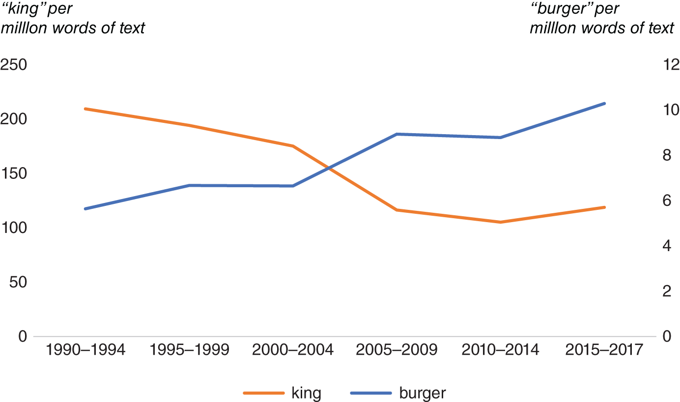
FIGURE 4.13 Frequency of the words “burger” and “king.”
Source: Based on data from Corpus of Contemporary American English.
4.6.9. Speech in NLP
Tasks involving speech are also part of NLP. For example, automatic speech recognition can also be considered as a part of NLP. Petkar (2016) discusses the many challenges associated with speech recognition. First, there is a difference between spoken language and written language. In some languages such as Arabic this can be very pronounced. There are large differences between the spoken dialects of Arabic and written text, which is in the form of Modern Standard Arabic. There are differences in pronunciation, vocabulary, and also grammar. However, even in English, spoken language tends to be less formal and generally less descriptive. The paper also notes the difficulties associated with continuous speech. Just as word segmentation needs to be performed on written text, for audio, speech segmentation is used to identify individual words, which can be challenging given that there aren't always clear pauses in human speech between words. There is also significant variability in speakers in terms of accent, gender, and speed of speech.
Speech recognition can often form the first step of solving an NLP problem, where our text is not in a written form. One example would be Siri, the Apple voice assistant on the iPhone, which takes the user's speech as an input. This is converted into written text, which is parsed for understanding using some of the techniques outlined earlier, into a structured form, so that we can understand things like the context. An answer is then generated based upon this structured input. The next step is natural language generation to create a human readable reply. Finally, text-to-speech synthesis is applied to this text to read aloud the output to the Siri user.
However, there are now new techniques that promise to apply advanced NLP techniques like translation from speech in one language into another, without intermediate conversion into written text and then application of text-to-speech synthesis. Jia and Weiss (2019) describe Translatotron, which uses a single sequence-to-sequence model for direct speech translation. The approach can even retain the style of speech from the original speaker, but in the foreign language, which would likely be more challenging to do using a traditional approach that requires a separate text-to-speech synthesis.
More broadly, we could argue that speech might have additional information that would be lost when converting into text. Speech has many different characteristics such as pitch, speed, and pronunciation that are not obvious from text. As a very simple example, it is far easier to determine the gender of the speaker from their speech than it is from reading their text. Features extracted from speech can be used to develop indicators for deception in speech and combined with text-based features. Hirschberg (2018) develops a machine learning–based approach for judging deception in speech, which outperforms humans.
From an investor viewpoint, many of these techniques are also relevant. Speech recognition could be used on events such as earnings conference calls and the question-and-answer sessions of central bank press conferences. Understanding deception in such situations would be extremely beneficial for investors, too! Text-to-speech could be used to provide automated alerts for traders, triggered by specific events like large price moves or economic events.
4.6.10. NLP Tools
What type of tools can we use to first get access to raw data from the web and then to structure it or to do tasks like automatic speech recognition? It is possible to develop libraries to do various NLP tasks such as generate word embeddings, word segmentation, sentiment analysis, and so on. However, it requires significant time and expertise to write these tools and then to train them.
In practice, there are many libraries and resources that can help us with different parts of the process that we can use as a starting point for our analysis of text. In many instances, these libraries also include models that have been pretrained on large corpora of text. Following is a list of some of the open-source Python tools available for the initial stage of gathering text data from the web and cleaning:
- Scrapy: Scrapy is a full framework for web crawling and web scraping. We can give it a URL and it will begin to crawl the various websites linked from that and help you save and download all that content.
- BeautifulSoup: BeautifulSoup focuses on parsing HTML data that has already been downloaded. Webpages have a large amount of formatting and script code, which are irrelevant for understanding the content. BeautifulSoup enables us to extract certain elements, remove superfluous information such as HTML tags, and so on. We can use Scrapy and BeautifulSoup together.
- PDFMiner: PDFMiner can extract text from PDF documents.
- tablula-py: tabula-py is a Python-based wrapper for the Java, Tabula library, specifically for reading tables from PDF documents. Use cases in finance could be reading from earning reports.
- newspaper3k: newspaper3k is a Python library for accessing articles from newspaper websites. It can, for example, extract the body text of articles and associated metadata such as the authors and publication date. It sits on top of some of the other libraries discussed here, like BeautifulSoup and NLTK.
Next, we list some of the libraries that are useful for higher-level natural language processing tasks, once we have gathered together and cleaned a text. We should also note that many of the general-purpose machine learning libraries such as TensorFlow and scikit-learn can also be used with text, although they are not specifically limited to dealing with text.
- NLTK: NLTK is one of the oldest Python libraries to do NLP tasks. It includes many trained models and word corpora to get you started, including a corpus of Reuters articles (from 1987). Bird, Klein and Loper (2009) guides users through using NLTK to a number of common NLP tasks ranging from processing raw text to text classification.
- CoreNLP: Stanford CoreNLP is accessible in a number of languages as well as Python. As with NLTK it performs a large number of NLP tasks, ranging from tokenization and sentence splitting to named entity recognition and sentiment tagging.
- Gensim: Gensim is a topic modeling library, which includes implementations of models such as Latent Dirichlet Allocation and Latent Semantic Analysis.
- spaCy: spaCy is written in Cython. It can do various NLP tasks such as tokenization, named entity recognition, and part-of-speech tagging. It also integrates with a number of Python machine learning libraries such as TensorFlow.
- pattern: pattern is a general-purpose web mining module for crawling the web and accessing sources like Twitter and Wikipedia via their APIs. It also contains a number of features to do NLP tasks, such as sentiment analysis based around words typically used in product reviews. It also includes functionality to perform simpler tasks such as part-of-speech tagging.
- TextBlob: TextBlob sits on top of NLTK and pattern. However, it provides an easier to use interface to access these libraries.
- BERT: BERT (Bidirectional Encoder Representations from Transformers) was developed by a team at Google; see Devlin, Chang, Lee and Toutanova (2018). Essentially, it is a method of pretraining language representations, which also incorporates context. It uses unsupervised learning, and as a result it can be trained on vast amounts of plain text. Google has a model that has been pretrained on text from Wikipedia and BookCorpus. The pretrained model can then be used for a number of NLP tasks such as question answering or tokenization. The software implementation of BERT uses Google's TensorFlow machine learning library.
- SpeechRecognition: SpeechRecognition is a Python library that allows users to do speech recognition using a number of external online and offline services using a common API.
While we have focused on open source Python tools, there are many commercial tools available for doing NLP on text. Many of these are cloud based and can be used as pay-as-you-go-style services, where you upload the text you would like to analyze, and then NLP is performed on it.
- Google Cloud Natural Language: Google Cloud Natural Language can do a number of NLP tasks, including named entity recognition, sentiment analysis, and syntax analysis. While it has pretrained models, users can also train their own custom models. It can be accessed using a REST API to upload text for analysis or it can also read text stored on Google Cloud. It also supports the creation of own custom models, or it can be used on own training data for content classification.
- Google Cloud Speech-to-Text: Google Cloud Speech-to-Text is a cloud-based service that can convert audio to text using neural network models, which has a number of different APIs. It supports 120 languages.
- Amazon Comprehend: Amazon Comprehend performs different NLP tasks on the provided text, extracting properties such as entities, syntax, and sentiment. It also has a specific version trained on medical vocabulary to extract data from medical notes or similar texts.
4.7. SUMMARY
Machine learning encompasses a large number of individual techniques. At its core it can be split up into supervised learning, unsupervised learning, and reinforcement learning. When fitting these models, we need to be aware of the variance-bias trade-off. What may appear to work very well in-sample can end up performing poorly in-sample, because we have overfit it.
In the chapter, we discussed a number of machine learning techniques ranging from relatively simple examples such as linear regression, to logistic regression for classification, to more complicated models such as deep neural networks. We also gave a short summary of some of the machine learning libraries that can be used to fit these models.
Later we discussed some of the limitations associated with machine learning, in particular with reference to financial time series, which are nonstationary. We also discussed specific use cases for structuring images, using techniques like CNNs and we also included an introduction to natural language processing, where machine learning models tend to be used these days, in preference to more traditional rule-based approaches.
In Chapter 13, we shall use a dataset of satellite imagery that has been structured using CNNs to generate car counts for the car parks of European retailers. In addition, we had a detailed look at natural language processing that can enable a computer to understand human language. In Chapter 15, we shall have an extensive look at text data, and give several investor use cases for it. For readers interested in machine learning in finance more broadly, we refer the reader to Lopez de Prado (2018) and also Dixon et al. (2020).
NOTES
- 1 See also Hastie (2009), Chapter 7.
- 2 We define complexity as the number of parameters in a model. The Vapnik–Chervonenkis (VC) theory provides a broader measure of complexity, see Vapnik (2013).
- 3 The contrary can be observed in specific situations.
- 4 Our prediction for
 is usually denoted
  .
. - 5 Typically, in binary output, we assign probabilities of more than
 to group
  and vice versa. For multiclass outputs, we usually assign to the class with the highest probability.
 - 6 Linear regression does not always assume a linear relationship between dependent and independent variables; we could have a model of
 and it is still considered to be linear regression.
 - 7 It is this prediction (read regression) of probabilities where logistic regression derives its name. We are merely extending it to a classification technique by deciding to assign a class based on this regressed probability.
- 8 Although, given that there are finite numbers of leaves on our trees, we cannot actually produce continuous predictions, but rather point out interval predictions along the real line.
- 9 For an introduction on CNNs, see Section 5.3.2.2
- 10 Some architectures, such as recurrent neural networks, allow nodes to feed back into themselves, other nodes in the same layer, or nodes in previous layers.
- 11 See Schaffer (1994) and Wolpert (2002).
- 12 See https://www.eff.org/ai/metrics for up-to-date performance benchmarks on different datasets. See Geirhos (2017) for different examples and comparisons of human vs machine performance under image degradations like contrast reduction, additive noise, or novel eidolon-distortions.
- 13 Long Short-Term Memory is an artificial recurrent neural network.
- 14 Bidirectional Encoder Representations from Transformers.
- 15 XLNet is a generalized autoregressive model for natural language understanding based on Transformers-XL
- 16 Sometimes, causality is not required, such as when counting cars in images or extracting sentiment from text. However, causality is necessary in macroeconomic forecasting, for example.
- 17 Cats do not change over time, especially after we observe them!