
CHAPTER 13
Satellite Imagery and Aerial Photography
13.1. INTRODUCTION
On October 4, 1957, the Soviet Union launched Sputnik I, the first artificial satellite in space. The first image of the earth captured by a satellite was made by NASA's Explorer VI Earth satellite (NASA, 2009) on August 14, 1959 (see Figure 13.1). The picture shows a sunlit area of the Central Pacific Ocean and its cloud cover. The photo was taken when the satellite was about 27,000 km above the surface of the Earth.
Of course, this was not the first time that Earth had been observed from the sky. During the First World War, for example, aerial photography became a significant weapon. While only a few hundred photos may have been taken in the first six months of the war, in 1918 Britain produced just over 5 million aerial photographs (Cable, 2015). And this was not the first example of aerial observation for military purposes. In the American Civil War, Thaddeus Lowe used a hot air balloon to perform aerial reconnaissance for the Union against the Confederate forces.
The most obvious difference between satellite imagery and aerial photography is the difference in altitude at which images are taken. From a much higher altitude, a satellite image will be able to capture a larger area. Furthermore, it can also capture weather patterns more easily and broadly. Satellites also regularly pass over the same spots, so they can potentially provide regular updates, and in effect in recent years this frequency has increased, given the number of satellites in the sky. At the same time, the cost of satellite imagery has come down. Overall, aerial photography tends to be more detailed. While in recent years the resolution of satellites has improved, there are limits to the resolution available on satellite images released to the public by law (Bump, 2017). Today there are many organizations in both the public and private domain that operate satellites for imaging purposes.

FIGURE 13.1 First picture from Explorer VI satellite.
Source: NASA.
There are difficulties associated with photographing the Earth from above, such as the vast amount of data generated, given the sheer size of the Earth's surface area and the resolution at which the images are captured. Also, we need to factor in issues like cloud cover, which at times can make some images less clear and usable. As with pretty much every other alternative dataset, the raw satellite imagery is essentially unstructured data. Hence, to be useful for investors it needs to be structured so it can be unified into a common format. Think about the way a human sees the world: we take in a large amount of information through our retina, then we dispense with much of that data and focus on just the important parts of the image.
Computer vision is the area that brings together many different techniques to help a computer see the world in a similar way to humans. There are several steps involved in computer vision, and we shall briefly describe some of these. The initial step deals with image acquisition, which involves the conversion of the world into a raw binary format such as through a digital camera. It should be noted that computer vision need not always deal with images that are observable to the naked eye. There could be data that includes wavelengths that are not visible to the eye, such as infrared wavelengths that allow night vision. There are also many transformations associated with computer vision that are used to enhance the original image, such as colorization, blur removal, or image reconstruction.
The second step is image processing. At this step the image is preprocessed and cleaned to prepare it for higher-level interpretation. This can include operations such as changing the contrast and sharpening the image, as well as the removal of noise and edge tracing. Applications that extensively use image processing algorithms include, for instance, Photoshop and Instagram. The final output of image processing is itself an image.
The next step involves analysis and understanding of the image, essentially being able to convert the image into text that can describe it. At the highest level, image recognition will try to understand the image as whole. Delving into specific parts of the image, object detection flags objects inside the image with a bounded box. Object classification and identification tags what the object is and its type respectively. For videos, these concepts can be extended to object tracking. Please see Chapter 4 for a more detailed discussion of computer vision.
From an economic or markets perspective, satellite imagery can give us a snapshot into the world in a relatively automated and cheaper manner that might be costly or difficult to gather using more traditional and manual methods. Obviously, the higher the resolution of a satellite imagery, the more content we will be able to detect and structure from an image. Furthermore, if we can capture the contents of a certain location repeatedly, we can build up a time series of data to measure changes in activity. Clearly, the more frequent our sampling of satellite imagery, the more expensive it will be to obtain and store the raw data. We also need to be aware of challenges like changes in weather, such as cloud cover, that affect how imagery is processed, and the fact that images are unlikely to be collected at regular intervals across every location of interest, given the way a satellite sweeps the ground.
In the following sections, we will discuss a number of different examples of using satellite imagery for economic applications. This will include the use of night light intensity to understand and forecast US export data, as well as more granular use of imagery to identify car park activity and estimate earnings for retailers' stocks.
13.2. FORECASTING US EXPORT GROWTH
Estimating export growth can be an arduous task. In practice, it is often measured by a proxy, namely the GDP of the foreign export partners of a country. As already discussed at length, the difficulty with GDP figures is that they tend to be recorded on a relatively infrequent basis, which is usually quarterly. There is also often a considerable lag associated with the release and subsequent revisions. Hence, by the time GDP data is released, this could be several months after the associated period it is actually measuring. If we can proxy foreign GDP with a timelier measure, we can in turn estimate foreign growth in the current quarter without a large lag (i.e. doing a timely nowcast). One proxy for GDP is to use PMI surveys (see Chapter 12). Here, we shall discuss an alternative approach.
Nie and Oksol (2018) discuss using satellite imagery as a proxy for foreign GDP and hence as a proxy for foreign US export growth. They focus on the measurement of nighttime lights from satellite imagery. The rationale is relatively intuitive. We would expect that as a country becomes richer and there is more economic activity, this is likely to be reflected in more night lights. They use a dataset of publicly available images through the Earth Observation Group at the NOAA (National Oceanic and Atmospheric Administration). They are filtered for specific “noise,” such as clouds. Each pixel on the image represents an area of around 1 square km. This type of resolution might be insufficient for measuring specific objects, such as cars or buildings. However, the focus here is simply on light intensity of a relatively big area. Each pixel has a value that represents night intensity between 0 and 63. Once a particular geographical area is identified, it becomes possible to create an index for measuring the light intensity of that area, whether it is a city, country, or other region.
TABLE 13.1 Annual correlation between exports, lights, and GDP.
Source: Federal Reserve of Kansas City, Haver Analytics.
| Variables | Advanced | Developing |
| Export growth and lights growth | 0.29 | 0.28 |
| Export growth and GDP growth | 0.79 | 0.49 |
| GDP growth and lights growth | 0.17 | 0.14 |
This way of proxying GDP, Nie and Oksol note, is particularly useful for emerging markets where official national statistics are likely to be less reliable. In Table 13.1, we present their results for annual correlations from 1993 to 2013, for export growth and light growth, export growth and GDP growth, as well as GDP growth and light growth. In advanced economies, there does appear to be a stronger correlation between export growth and GDP growth. However, this correlation is weaker for developing economies. The authors conjecture that this is because GDP is better measured in advanced economies compared to developing economies.
Later, Nie and Oksol construct quarterly models to estimate export growth in the current quarter: a random walk model, a GDP model, and a light-based model. They note that while GDP data is only available quarterly, light data in recent years has become available on a monthly basis (and since 2017 on a daily basis). Hence, they repeat the exercise for a monthly random walk model and also monthly light models to estimate export growth.
They then compute the average percentage derivation between the model estimates and actual data, which we show in Table 13.2. It is notable that the monthly-based lights model outperforms all the other models, across all economies, for forecasting US export growth. This suggests that night light data could indeed be a useful way to help estimate export growth in a timely fashion, in particular where GDP data is lagged.
TABLE 13.2 Comparing model forecasts through the average percentage derivation at quarterly and monthly frequency.
Source: Federal Reserve of Kansas City, Haver Analytics.
| Model Specification | All | Advanced | Developing |
| Random walk: quarterly | 2.2 | 3.23 | 4.13 |
| GDP: quarterly | 2.89 | 3.06 | 4.06 |
| Lights: quarterly | 3.06 | 4.05 | 3.11 |
| Random walk: monthly | 2.28 | 2.14 | 3.27 |
| Lights: monthly | 1.33 | 1.28 | 2 |
13.3. CAR COUNTS AND EARNINGS PER SHARE FOR RETAILERS
Imagine that you want to understand the retail sales of a certain store or the number of diners frequenting a certain restaurant. One way to get an idea is to count the number of customers walking inside the store or restaurant. If a store has only one entry and exit, it might be feasible to do this manually. However, if we are talking about a large store with lots of entry points and many branches in different parts of the country, it ends up being a logistic nightmare. If we want to track the whole retail sector, it quickly becomes a very big undertaking to source such data and manage the processes behind. Alternatively, we can attempt to automate the problem by using satellite imagery. Satellite images of car parks attached to the stores can be used as input data for this purpose.
We have explained earlier in broad terms (see Section 4.5) how it is possible to classify an image or objects by using a number of techniques. In particular, we noted that using a convolutional neural network outperforms more traditional classification techniques. Whatever the chosen technique, the goal is to structure the images and extract the relevant information. This would usually involve identifying and counting the number of cars in each of these satellite images, using techniques such as convolutional neural networks. The hypothesis to be tested is that the number of cars at any one time would be a proxy for retail activity in a store or how busy a restaurant is. Potentially, we might expect that this could be a good indicator for the earnings reported by the firm. In order to do this, it is necessary to have satellite images of sufficiently high resolution. This contrasts with our earlier example of measuring nighttime light intensity, which may be possible using lower-resolution imagery. Furthermore, as with any satellite imagery, there can be the additional complications of factors such as cloud cover, which can impact the analysis and the conclusions drawn from an image.
The car counts are, of course, only going to be an approximation, given that we do not really know the spend per customer from a satellite image. Furthermore, this approach is also most appropriate for those retail outlets whose customers are mostly driving there by car. Of course, although we are here focusing on retail outlets or restaurants, we could apply the techniques to any other consumer-oriented business.
In order to make these car counts useful, extra data is required that is not contained in the image, such as address data, which we can join with the geospatial data. In particular, once we have the address of each car park in every image, we can focus on those car parks that are adjacent to particular retail outlets and ignore other car parks. If our goal is to use this data for trading purposes, we need to do some entity matching. In other words, we also need to be able to match the various retail brands of the car parks to their underlying equities, which we can trade. Indeed, this type of joining with other datasets and entity matching is a common feature of most alternative data use cases, as we have already explained in Chapter 3.
To test this hypothesis, we use a dataset from Geospatial Insight derived from satellite imagery data. Geospatial Insight has access to a network of more than 250 satellites in orbit for gathering their imagery. They primarily use Digital Global Worldview's network of satellites. The resolution of the images produced by these satellites is particularly high (26cm–51cm). This level of detail enables the identification of cars, but not, for example, number plates or people.
Our focus is on Geospatial Insight's RetailWatch dataset, which we shall use to estimate company performance for several European retailers. It consists of the number of cars parked nearby several retail outlets in Europe, with observations snapped on a regular basis. From the input images, areas bounded by the geofenced outlines for specific retailer car parks of interest are clipped. A convolutional neural network (CNN) predicts the likely location of cars within these clipped car park areas, which has been trained on a large dataset of manually annotated car positions. Post processing then extracts the individual car locations, and a car count is constructed from that for each car park area. While the process is automated, manual checks are also done to check the accuracy.
The dataset currently tracks a number of publicly traded companies, as well as a number of additional private companies. While there are a few datasets for the car parks of similar retailers based in the United States, such as Walmart, at the time of writing it is less common to find ones that are specifically focused on Europe. For obvious reasons such an approach is not going to be as useful for purely online-focused retailers. Instead, for those types of firms we would need to use other approaches, like examining consumer transaction data.
The focus of our study will be on the retail outlets attached to firms that are publicly traded on equities markets. For each company, the raw data provided by Geospatial Insight consists of the company name, the associated equities' Bloomberg ticker, as well as the name and location of the retail outlet car park. There is a timestamp for each observation, with the area of the car park and the number of cars counted. The dataset is relatively sparse, since we do not necessarily have observations every single day. As we might expect from satellite data, the observations on a particular day are not all snapped at the same time. Given the way that satellites sweep over the sky, they will be covering different parts of the earth at different times. It is also the case that the number of car parks photographed can vary significantly at any day. There can also be issues associated with cloud cover. Chapter 8 presented a case study of how to impute missing points in satellite imagery of car parks.
We go through several steps to compute an indicator based on car counts:
- We compute the total amount of area photographed and the number of cars counted during that period on a rolling basis.
- In order to adjust for the fact that the images will vary in terms of the car parks being photographed for a certain retailer, we compute the ratio of the cars counted divided by the total car park area photographed. If we do not do this, then we will end up overcounting those days when more images happened to be collected.
- Obviously, there are other ways to combine the data. At present we are ignoring any store-by-store differences, and we instead aggregate all these observations into one variable. We could instead try to combine the car count data at the store level first, and then include these as separate variables in any model. We could also try to classify stores according to the relative size of their car parks, and aggregate them for “small,” “medium,” and “large” stores, using these car counts as different variables in our model.
Our current approach does take into account the relative size of the car parks for each store (as proxied by the total car park area). However, it does not use any other metadata associated with the store, such as location. We also do not bucket specific stores together by other metrics, such as the car park size. The difficulty with aggregating at a very high granularity is that our dataset might become too sparse. Hence, any sort of bucketing would need to take this into account. It is also the case that the irregularity of snapshots might pose problems. For example, it is unlikely to be a good approach to compare a specific store with snapshots taken at very different times of day. Other issues such as cloud cover could also prove more problematic for this type of approach.
Given our hypothesis that car count data can be a good proxy for earnings, we can take a rolling average that matches with the official earning announcements for each firm. This will also help to smooth out the sparseness of the data. Typically, a publicly traded firm will have earnings announcements at quarterly intervals, twice a year or annually. The benefit of our car count dataset is that we will have it as soon as the period has finished, well before the official announcement. It has been well known for many decades that equities experience a post-earnings announcement drift, so if earnings are better than expected, typically the stock goes higher in the immediate aftermath and falls on disappointing earnings (Ball & Brown, 1968).
Hence, if our car count measure can be used to enhance earnings forecasts, we can potentially trade the associated equity around earnings announcements. If we forecast higher earnings than the market consensus, we buy the stock before the announcement and take profit afterwards. Alternatively, our car-count-enhanced earnings forecast could potentially be used as an additional factor in cross-sectional long/short equity baskets.
In our case, the European retailers within our car park dataset generally report semi-annually. Therefore, we create 6-month rolling averages of our adjusted car count measure. We can then snap the value that corresponds to the reported earnings periods. A major benefit of using the car count data is that it is available as soon as the earnings period ends. This contrasts to the reporting of earnings, where there is likely to be a lag of a few weeks. The earnings consensus is also available before the actual official earnings announcement. However, it is likely that it will change in the leadup to the announcement, as analysts update their estimates. Hence, earnings consensus estimates are unlikely to give you as early an indication as measures purely based on car count.
However, does our car counting measure have any relationship with the actual earnings per share announcement and the earnings consensus, as compiled by Bloomberg, for example? Figure 13.2 plots our car count measure for Marks & Spencer, against both the announced earnings per share and the estimate. At least in this stylized example, it does appear that our car count measure derived from satellite imagery of Marks & Spencer's car park does appear to be strongly correlated with both the consensus estimate and the actual announcement. Admittedly, we have relatively few data points in our history. One way to help expand our study is to look at more companies, which we shall do later.
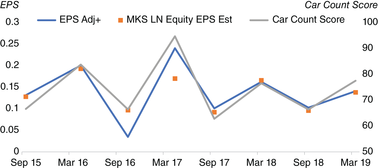
FIGURE 13.2 Car count for Marks & Spencer versus earnings (actual and estimate).
Source: Based on data from Geospatial Insights, Bloomberg.
Does using the car count data have additional insight compared to using the consensus? To check this historically, we look at several companies in the dataset, where we also have a full set of Bloomberg consensus data. We create several full sample linear regressions, to help predict the earnings per share, which is our dependent variable ![]() . The first regression uses only consensus data as its independent variable
. The first regression uses only consensus data as its independent variable ![]() . The second regression uses the car count score
. The second regression uses the car count score ![]() as its independent variable. The last regression uses both consensus data
as its independent variable. The last regression uses both consensus data ![]() and car count score
and car count score ![]() as its independent variables. In Figure 13.3-2, we report the adjusted
as its independent variables. In Figure 13.3-2, we report the adjusted ![]() of these regressions for several UK retailers.
of these regressions for several UK retailers.
We see that, in all cases, adding car count data to consensus helps to increase the adjusted ![]() , compared to using the consensus alone. This suggests that there might indeed be value in using car counts as an additional variable to consensus when forecasting earnings.
, compared to using the consensus alone. This suggests that there might indeed be value in using car counts as an additional variable to consensus when forecasting earnings.
Of course, there are some caveats to our analysis that we need to mention. The data history in the study is relatively small from 2015 to 2019. In Figure 13.3, we have only three companies. We could source consensus estimates from other sources to help add other companies within the Geospatial Insight dataset into our study. Furthermore, another caveat is that we are trying to use the data to help forecast only a handful of points and then calculating our in-sample regressions with a very small sample set. However, as history accumulates, this is going to be less of a problem.
We have seen that adding car count data to consensus estimates can be helpful for explaining earnings per share. What if we explore combining car count measures with another alternative dataset, such as news? Furthermore, this will enable us to compare car counts with news. As with car counts, news-based measures will be available as soon as the earnings period ends, rather than being lagged, or only being fully updated close to actual earnings release. This contrasts to consensus data that is only going to be fully updated very close to the earnings call. If we want an earlier forecast for earnings, we need to focus on those datasets that are available well before the actual earnings announcement.
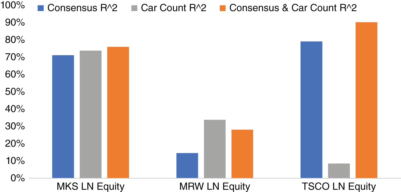
FIGURE 13.3 Regressing consensus and car count data with earnings per share for the period September 2015–March 2019.
Source: Based on data from Geospatial Insight, Bloomberg.
For a news-based measure, we use indicators that record the number of news articles from Bloomberg News for given publicly traded equity tickers. The indicators are split between the number of positive and negative news articles published for each company. We compute a rolling average of the number of positive stories minus the number of negative stories, which corresponds to the length of report period to create a news sentiment metric.
We snap the value of the rolling news metric indicator at the end of each reporting period. Hence, the approach is somewhat similar to the way we treat our car count measure. We expand our universe for all the publicly traded companies in the RetailWatch dataset, even those for which we do not have a full set of consensus data, given that we are not using that in this instance.
We again create several full sample linear regressions, to help explain the actual earnings per share, which is our dependent variable ![]() . The first regression uses only our news indicator as its independent variable
. The first regression uses only our news indicator as its independent variable ![]() . The second regression uses only our car count as its independent variable
. The second regression uses only our car count as its independent variable ![]() . The last regression uses both the news indicator
. The last regression uses both the news indicator ![]() and the car count score
and the car count score ![]() as its independent variables. In Figure 13.4, we report the adjusted
as its independent variables. In Figure 13.4, we report the adjusted ![]() of these regressions for a number of European retailers. We note that since publication, Geospatial Insight have added a large number of additional tickers to the RetailWatch dataset.
of these regressions for a number of European retailers. We note that since publication, Geospatial Insight have added a large number of additional tickers to the RetailWatch dataset.
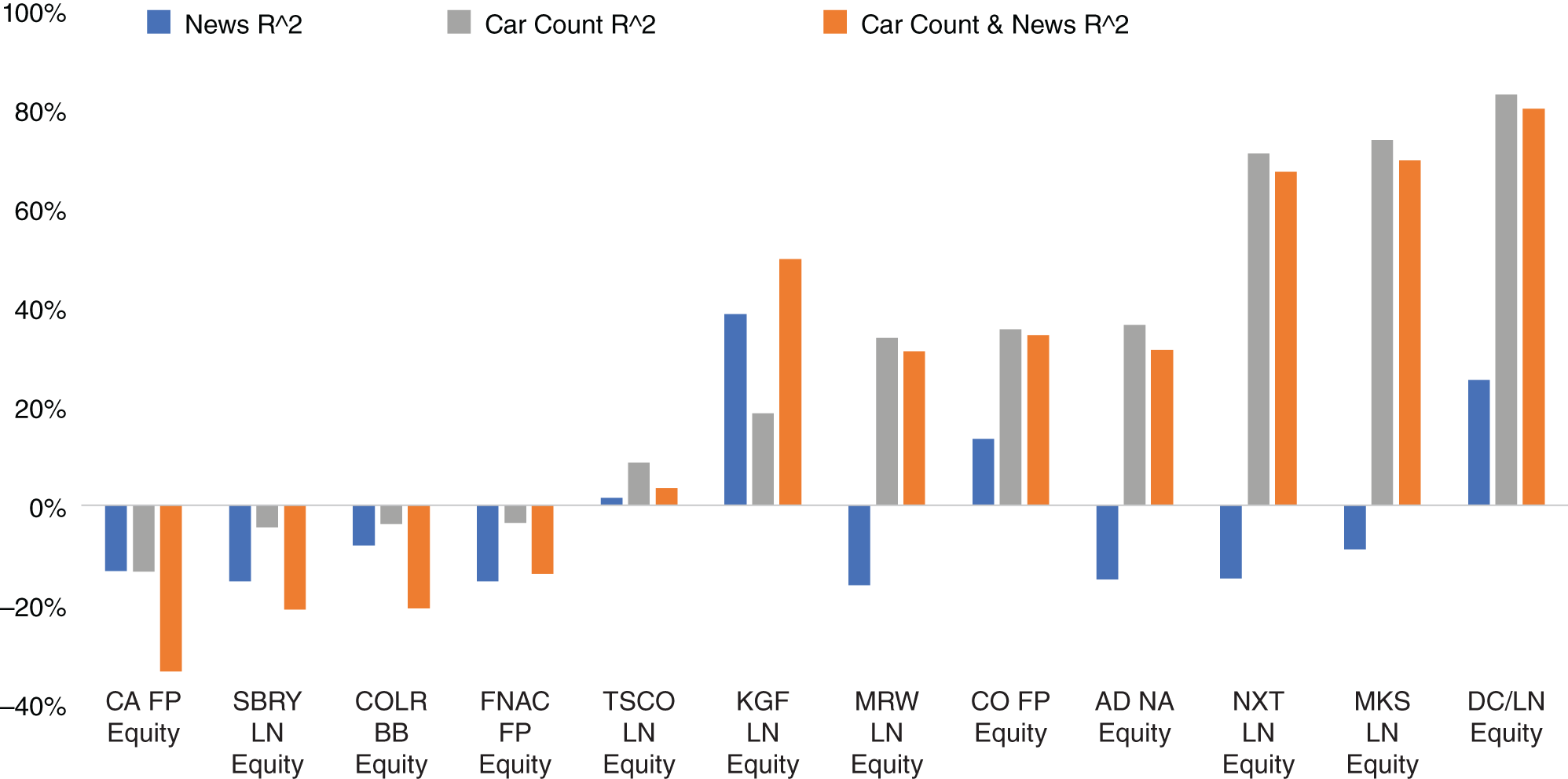
FIGURE 13.4 Regressing news sentiment and car count data with earnings per share for the period September 2015–March 2019.
Source: Based on data from Geospatial Insights, Bloomberg.
For a small number of companies such as Carrefour (i.e. CA FP Equity), both car count and news sentiment metrics have quite low adjusted ![]() . There can be many explanations for this. It might be the case that many customers visit their stores by public transport, or indeed that news sentiment is relatively neutral; hence it is difficult to extract a directional signal.
. There can be many explanations for this. It might be the case that many customers visit their stores by public transport, or indeed that news sentiment is relatively neutral; hence it is difficult to extract a directional signal.
In the majority of cases the adjusted ![]() of car counts is higher than the adjusted
of car counts is higher than the adjusted ![]() news sentiment, when regressing each variable separately against earnings per share. We find that, in general, adding news does not help to increase the adjusted
news sentiment, when regressing each variable separately against earnings per share. We find that, in general, adding news does not help to increase the adjusted ![]() of car counts alone, other than Kingfisher (KGF LN Equity). Later in the book we will show that there are instances where news can be used to trade markets profitably, in particular FX, on a historical basis. However, this is typically by aggregating the news on a shorter time horizon, rather than using it to forecast EPS by looking at it over a very long period of time (6 months).
of car counts alone, other than Kingfisher (KGF LN Equity). Later in the book we will show that there are instances where news can be used to trade markets profitably, in particular FX, on a historical basis. However, this is typically by aggregating the news on a shorter time horizon, rather than using it to forecast EPS by looking at it over a very long period of time (6 months).
In summary, we have used relatively simple techniques for aggregating the car count data and even with these very few basic and intuitive steps we have seen that the car count method shows promise. Further work could include using the same technique but on other datasets, covering, for example, other developed economies like the United States and Canada. Also given that the dataset reports for individual car parks for each company, it would be worth investigating whether certain car parks act as leading indicators for the broader company. We have also noted that augmenting the car count indicator with other metrics such as the consensus earnings estimates or news sentiment–based indicators can increase in certain cases the overall explanatory power when it comes to understanding earnings per share. However, the lack of plentiful history in the dataset impedes drawing strong statistical conclusions for the time being.
It is also worth exploring whether consensus earnings estimates can be combined with other alternative datasets (in addition to news as we have done), such as consumer transaction data or mobile phone location, to create more accurate forecasts for earnings. In practice, all these measures are only taking partial samples of consumer spending patterns or general sentiment toward a firm. Hence, by increasing the size of our sample using more alternative datasets, we are likely to increase accuracy provided the samples do not totally overlap.
13.4. MEASURING CHINESE PMI MANUFACTURING WITH SATELLITE DATA
In Chapter 12, we discussed PMI data at length, noting that this survey-based “soft” data can be a leading indicator for GDP, which is “hard data.” One question we may wish to ask is whether we can create a leading indicator for PMI data using another alternative dataset, such as satellite imagery. Such an estimate is likely to be available before PMI data is compiled and released.
For certain types of economic activity, like industrial activity, it seems intuitive that a physical imprint could be left behind that can be profitably exploited. After all, manufacturing processes often require the ingesting of raw materials, which are likely to be stockpiled, in order to create finished goods that can also be tracked. This contrasts to an industry like finance, which is less likely to leave behind a physical imprint as an exhaust of its activity. Also, for some parts of the world, official economic data might not be as reliable or may be released with very large lags. Hence these alternative ways of measuring economic activity could be particularly useful, as we already discussed at length.
Eagle Alpha (2018) discusses the usage of satellite imagery by SpaceKnow to estimate Chinese PMI manufacturing data. SpaceKnow tracks specific signs of industrial activity, such as new construction sites or the accumulation of inventory. Over the 14-year history, 2.2 billion observations have been collected to generate the dataset over an area of over half a million square kilometers.
The Normalized Difference Vegetation Index (NDVI) has been created to understand how much vegetation covers the Earth's surface (Weier & Herring, 2000). Vegetation absorbs visible wavelengths of light, for use in photosynthesis, but tends to reflect infrared light to reduce the chances of overheating. By contrast, soil tends to absorb less visible light. Clearly, as a result, vegetation tends to appear lighter to the naked eye while soil is darker. The Enhanced Vegetation Index (EVI) works in a similar way but corrects for distortions in reflected light because of particles in the air.
SpaceKnow uses a similar approach in their algorithm, albeit for identifying the coverage of man-made structures as opposed to vegetation. The general idea behind their algorithm is that cement and steel reflect on the surface light of different wavelengths in a specific way. Hence, just like with the NDVI, it is possible to identify how much of the surface is covered with cement and steel structures. The algorithm also adjusts for various atmospheric factors that are likely to impact the image, such as cloud cover or aerosols. The algorithm compares the images from over 6000 industrial facilities to create SpaceKnow's satellite manufacturing index (SMI). The SMI is released every Monday, Wednesday, and Friday with a 10-day lag, compared to both official and Caixin PMI indices, which are published monthly with a 1-month lag.
The focus of China's official PMI manufacturing is larger firms, including state-owned enterprises. Caixin's PMI, on the other hand, focuses on small and medium-sized firms. Figure 13.5 shows China's official PMI manufacturing index, Caixin PMI manufacturing, alongside SpaceKnow's satellite manufacturing index. At least from a cursory glance, there does appear to be a good relationship between SMI and the other the other PMIs, despite the fact that the source data is, of course, very different. The correlation between SMI and China's official PMI manufacturing is 64% in our sample.
From a trading perspective, if we are forecasting an economic indicator, such as PMI, we might be interested in understanding how it compares with consensus forecasts, compiled by firms such as Bloomberg from a number of market economists, usually in sell-side firms.
At least in the very short term, the market reacts to surprises versus market expectations. If the market is already expecting a very bad number, and the release is indeed a very bad number, it is likely that the market reaction will be muted. We illustrate this point in Figure 15.5, where we give an example of how USD/JPY reacts to the surprise in nonfarm payrolls. In this instance, the relationship is broadly linear between short-term returns and the surprise (at least for relatively small surprises). Hence, it suggests that if we are able to understand the nature of the data surprise, we might be able to monetize it.

FIGURE 13.5 China SpaceKnow's satellite manufacturing index versus official Chinese PMI manufacturing and Caixin PMI manufacturing.
Source: Based on data from SpaceKnow, Bloomberg.
Does the SMI give us any further information compared to using the consensus forecast in isolation? Our focus is on forecasting the official China PMI manufacturing dataset, given that it has a much longer history available both for the actual data and the consensus forecast from Bloomberg.
In order to answer our question, we create a hybrid model. Our model uses a rolling linear regression, as seen in Equation (13.1), which has an expanding window. Our independent variables are the consensus forecast ![]() and the SMI
and the SMI ![]() . Our dependent variable
. Our dependent variable ![]() is the actual Chinese PMI manufacturing data release,
is the actual Chinese PMI manufacturing data release, ![]() is the constant of the regression, and
is the constant of the regression, and ![]() is the error. Thus:
is the error. Thus:
We use last month's coefficients from this model to create a forecast of the current month of Chinese PMI manufacturing. We use current month points for SMI and the consensus forecast for our independent variables.
In Figure 13.6, we plot the surprises in China PMI manufacturing versus the consensus from Bloomberg, SMI and also our hybrid model, during our sample, which runs from 2011 to early 2019. The worst performer is SMI, which has a mean absolute error of 1.05. The mean absolute error for the consensus surprise is 0.42, which is virtually the same as the hybrid model.
We might therefore question why we would use the satellite data, if the consensus model provides virtually the same mean absolute data with or without including it. We noted earlier that the satellite data is available ten days before the actual China PMI manufacturing release. We have used the final consensus number, which is updated just before the actual release. The consensus number will often change as we approach the actual economic release, as economists update their forecast in the survey. Hence, it is likely that ten days before the event we would not have a fully updated consensus number whereas we would have the SMI data point. Furthermore, the SMI data is also published on a high-frequency basis, every Monday, Tuesday, and Wednesday. By contrast, China PMI is only published once a month.
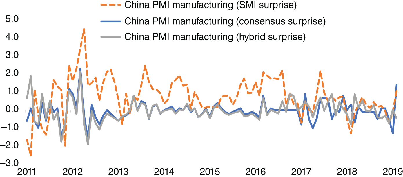
FIGURE 13.6 Surprises in China PMI manufacturing versus consensus, SMI and hybrid.
Source: Based on data from SpaceKnow, Bloomberg.
It also is possible that in practice we could improve upon the hybrid model by adding more variables to reduce the mean absolute error. In other words, it may be possible to augment observations made from existing datasets, rather than using them as a replacement. We would, of course, caution that mean absolute error should not be the only metric by which we judge a forecast. We could also try to backtest a trading strategy based on the SMI indicator, too, as another way to test its value. Furthermore, we could try to use SMI to model other indicators, in particular hard data, which are released later.
13.5. SUMMARY
Data derived from satellite imaging and aerial photography has been used for many years, particularly in the military sphere. In more recent years, alternative datasets have been developed by using satellite and aerial photography for investors. We have described several such datasets, including Geospatial Insight's dataset for car counts in the parking lots of European retailers, which we have used to estimate earnings per share data with good results. We also showed how using several datasets together could help to improve the explanatory power of a model for estimating earnings per share (for example, here with news sentiment data on the same retail stocks).
Key to all these image-based datasets is the use of efficient structuring techniques to convert the satellite image into a more usable, usually numerical form that can be more easily consumed by investors. Techniques such as convolutional neural networks have proved very effective for tasks such as object detection in images (see Chapter 4, for a further discussion on using machine learning to structure images).
However, the usage of satellite data as an alternative dataset is a pretty recent phenomenon that translates into short-length datasets. This issue is, of course, temporary, and soon we will have enough imagery data to make statistically robust models and conclusions.