
CHAPTER 12
Purchasing Managers' Index
12.1. INTRODUCTION
As we discussed in Chapter 1, the ability to accurately predict changes in key economic indicators, such as GDP, can serve a wide number of groups, not only investors. We mentioned that PMI indicators could be a good proxy for this purpose. Given their importance, in this chapter we will elaborate more around them. We will present some quantitative analysis to justify their use.
GDP forecasting (or better nowcasting) can be used by policymakers to optimize changes to key macroeconomic management levers such as interest rates or fiscal policy. Likewise, by knowing the current macroeconomic context, investors and businesses can make investment allocation decisions with greater certainty and potentially better performance. As a result, in recent years, practitioners have focused on improving their understanding of economic performance in near “real time,” rather than waiting for updates to slowly produced official figures, such as GDP, which are also numbers subject to notable future revisions. Performing such a task requires the use of other high-frequency datasets that are released in a timely fashion. This up-to-date information can be exploited to predict, or nowcast, slower-released, low-frequency macroeconomic variables such as GDP.
For example, the PMI series produced by IHS Markit in over 40 countries can be such a high-frequency and timely data source. It is derived from a questionnaire sent to a fixed panel of selected business executives across both manufacturing and service-sector industries. The PMI datasets provide monthly information on a wide variety of metrics such as output, new orders, employment, prices, and stocks. Hence, the PMI datasets provide an insight into countries' current and expected level of business activity. They can also be a leading indicator to forecast upcoming expansions or recessions.
The advantage of the PMI is that it is released earlier than other official indicators, such as the industrial production index or GDP. Typically, they are conducted in the middle of the month. Results from the surveys are released on either the first day (manufacturing) or third working day (services and composite aggregations of both sectors) following the reference period. However, for the eurozone (plus the US, UK, Japan, and Australia), PMI “flash” data is also available around 10 days before the “final” releases. These flash numbers are based on around 85%–90% of the final sample and the revisions between “flash” and “final” PMI data is typical but usually small. In the Eurozone, detailed flash PMI figures for France and Germany are also provided.
Figure 12.1 shows how the PMI data fit into a typical timeline for nowcasting GDP growth in a given quarter (in this example, Q2 2018).
To highlight the relative timing advantage of the PMI, the release formats of two closely watched indicators – the European Commission's Economic Sentiment Indicator (ESI) and official figures from Eurostat on industrial production – are also provided.
The Economic Sentiment Indicator, abbreviated as ESI, is a composite indicator made up of five sectoral confidence indicators with different weights: (1) industrials confidence indicator (40%), (2) services confidence indicator (30%), (3) consumer confidence indicator (20%), (4) retail trade confidence indicator (5%), and (5) construction confidence indicator (5%). The economic sentiment indicator is published monthly by the European Commission. The ESI is derived from surveys gathering the assessments of economic operators of the current economic situation and their expectations about future developments.1
The timeline in Figure 12.1-1 provides an indication of how data availability builds through a nowcasting cycle: during the first two months of a quarter, only survey (so-called “soft”) data is available – the PMIs and the ESI. It is not until midway through the final month of the quarter that official “hard” figures (in this case industrial production) are available for the first month. So, until a certain point, economists, investors, and policymakers are reliant on soft data to gauge economic performance. Indeed, it is the non-synchronization of releases and subsequent timing advantages that the PMI tends to enjoy that provides the foundation for its use, especially in areas such as monetary policy.
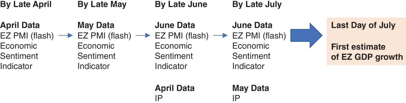
FIGURE 12.1 Nowcasting Eurozone (EZ) GDP Growth in Q2 2018.
Source: IHS Markit.
12.2. PMI PERFORMANCE
Being of a higher-frequency and timelier nature than GDP statistics, PMI datasets can be a good candidate to meet the demands of continuous tracking of economic growth. In Figure 12.2 we can observe the relationship between quarterly changes in GDP and the PMI for the Eurozone.
Since 2006, the Eurozone Composite PMI (which combines the manufacturing and service sectors) has correctly indicated underlying changes in growth through the financial crisis in 2008–2009, the Eurozone debt-crisis intensification in 2011, and the 2017 upswing in economic performance. Table 12.1 shows correlation statistics for the Eurozone, and its three largest member states. The comparison period begins in January 2000, but to provide a sense of performance since the depths of the 2008–2009 global financial crisis, we also provide a subsample of results since January 2010.
Generally speaking, the PMI outperforms the ESI and is comparable to industrial production at the Eurozone and country level. Naturally there are some exceptions, with industrial production data in Germany notably a strong performer, perhaps not surprising given the structure of Germany's economy. These results also hold broadly true since January 2010, with the PMI performance for Italy especially eye-catching. France remains a laggard in terms of pure correlation statistics, although the PMI continues to perform better than the respective ESI and industrial production data series.

FIGURE 12.2 Eurozone GDP and Composite PMI.
Source: Based on data from IHS Markit, Eurostat.
TABLE 12.1 GDP Growth correlations with % changes of select indicators.
Source: Based on data from IHS Markit.
| Euro area | France | Germany | Italy | |
| Since Jan 2000 | ||||
| PMI Comp | 0.87 | 0.57 | 0.76 | 0.79 |
| EC ESI | 0.76 | 0.41 | 0.61 | 0.7 |
| IP | 0.88 | 0.55 | 0.86 | 0.82 |
| Since 2010 | ||||
| PMI Comp | 0.84 | 0.52 | 0.64 | 0.89 |
| EC ESI | 0.71 | 0.46 | 0.32 | 0.74 |
| IP | 0.74 | 0.41 | 0.79 | 0.7 |
12.3. NOWCASTING GDP GROWTH
We now turn to the short-term predictive power of the PMI (as well as the ESI and industrial production) in forecasting quarterly changes in GDP via a simple nowcasting exercise. To circumvent the issues of misaligned time frequencies (PMI data are released monthly and GDP quarterly), we base our nowcasting model on a simple AR-MIDAS (mixed-data sampling) style regression. It is a single-equation approach, where quarterly GDP is explained by specifically weighted observations of monthly predictors. In mathematical terms:
In this broadly standard forecasting setup, current quarter ![]() is predicted by using a lag of itself
is predicted by using a lag of itself ![]() and a weighted average
and a weighted average ![]() of an explanatory variable
of an explanatory variable ![]() . There are k = {1,…, m} observations of X seen over the time period t (in this instance k = 3, which is the number of monthly observations of the explanatory variable recorded per calendar quarter).2
. There are k = {1,…, m} observations of X seen over the time period t (in this instance k = 3, which is the number of monthly observations of the explanatory variable recorded per calendar quarter).2
We run the model as an out-of-sample nowcasting exercise for the period 2010Q1 to 2018Q1. We use both the PMI and the ESI separately as the variable ![]() . For industrial production data, the process is simplified by creating a quarterly series of 3m/3m changes and regressing this (along with a lag of the dependent variable) against GDP. Note, however, that the industrial production data is based on “pseudo-time,” meaning that when predicting GDP growth, we assume that industrial production data are only available for the first two months of a quarter (as would be the case in a real-time GDP exercise). In essence, this means a time shift of a quarterly industrial production series is performed, whereby month-two observations are used in the regression exercise.
. For industrial production data, the process is simplified by creating a quarterly series of 3m/3m changes and regressing this (along with a lag of the dependent variable) against GDP. Note, however, that the industrial production data is based on “pseudo-time,” meaning that when predicting GDP growth, we assume that industrial production data are only available for the first two months of a quarter (as would be the case in a real-time GDP exercise). In essence, this means a time shift of a quarterly industrial production series is performed, whereby month-two observations are used in the regression exercise.
TABLE 12.2 Model performance (2010Q1–2018Q1).
Source: Based on data from IHS Markit.
| BM | PMI | ESI | IP | |
| Euro area | ||||
| RMSFE | 0.3 | 0.23 | 0.34 | 0.28 |
| Correct (%) | 82.8% | 72.4% | 65.5% | |
| France | ||||
| RMSFE | 0.39 | 0.32 | 0.42 | 0.21 |
| Correct (%) | 59.4% | 56.3% | 81.3% | |
| Germany | ||||
| RMSFE | 0.62 | 0.5 | 0.62 | 0.39 |
| Correct (%) | 68.8% | 56.3% | 78.1% | |
| Italy | ||||
| RMSFE | 0.31 | 0.29 | 0.34 | 0.44 |
| Correct (%) | 69.0% | 69.0% | 65.5% |
To compare nowcasting performances, the Root Mean Square Forecasting Errors (RMSFE) and the percentage of correctly predicted changes in GDP are provided. In the case of RMSFE, readings closer to zero should be viewed as the most positive. For added context, we also provide the results of a simple benchmark model (denoted as “BM”), which is simply a “no-change” forecast (i.e. current quarter GDP growth is assumed to be unchanged since the previous observation). Table 12.2 provides a summary of the various model performances.
The results show that, in nowcasting terms, models that include PMI data generally outperform those based on the ESI when it comes to predicting quarter-on-quarter growth rates. This is especially the case at the Eurozone level, where the PMI-based model outperforms equivalent ESI and industrial production set-ups considerably in terms of RMSFE while also registering a near 25% average nowcasting gain over the benchmark model. Moreover, the PMI model correctly forecasts the direction of quarterly growth in the Eurozone over 80% of the time (again a better result than what is seen for the ESI and industrial production).
For France and Germany, PMI-based models again outperform the simple benchmark and ESI models – and indicate the value-added of using PMI when it comes to predicting GDP growth – but it is the industrial production–based models that perform the strongest in terms of RMSFE and forecasted direction (though of course the delay in the publication of the industrial production data relative to the PMI needs to be borne in mind here). In Italy, it is only the PMI that outperforms the benchmark based on the RMSFE statistic.
12.4. IMPACTS ON FINANCIAL MARKETS
Having shown the predictive power of PMIs for GDP, we now turn to examine their impact on financial markets, which is the main interest of investors.
As Gomes and Peraita (2016) point out, one of the main problems in measuring the effects of economic indicators on financial markets is that both sets of data are usually available at different frequencies. Although financial data can be obtained for daily, hourly, or even finer intervals, macroeconomic indicators are produced and released at most monthly. Historically this led to the formation of two strands of thinking when modeling the relationship between macroeconomic information and financial markets. One strand consists of the use of lower-frequency regression by aggregating the financial market variables to a less granular time scale (e.g. calculating stock returns at monthly frequency and then regressing on monthly macroeconomic variables). The other strand consists of performing an event study analysis of the impact of a macroeconomic announcement on financial markets at the moment immediately after this information is released. For example, this could be payroll data numbers publication and its effect on stock markets. Gomes and Peraita (2016) provides a good literature review of different studies belonging to the two strands. Their study, however, focuses on the second.
Gomes and Peraita (2016) analyze the effect of PMI announcements on stock market returns and sovereign bond yields for Germany, France, Italy, and Spain, and on the Euro exchange rate, for the period between 2003 and 2014. They find that all of the examined financial markets are affected by the Purchasing Managers' Index announcements, in particular by negative announcements during the Euro Area crisis. Markets that experience the greatest impact are the stock markets, and these are particularly impacted by negative surprises in the PMI announcement. They also find that the effect on bond markets is of a lower magnitude and is symmetric and that the impact of the PMI in most financial markets became significant after the beginning of the crisis in 2008.
Hanousek and Kočenda (2011) analyze the effect of PMI indices on the stock markets of three EU countries – Czech Republic, Hungary, and Poland. They find that PMIs impact the markets in an intuitive manner: a worse-than-expected outcome provokes a negative effect on stock returns and vice versa. The analysis in the papers of Gomes and Peraita (2016) and Hanousek and Kočenda (2011) are both based on the news “surprise” (i.e. the deviation between expectations and the announced PMI). More formally, following the approach of Andersen (2007), they use the following definition of “surprise”:
where ![]() denotes the announced value of an indicator and
denotes the announced value of an indicator and ![]() refers to the market's expectation of that indicator at time
refers to the market's expectation of that indicator at time ![]() .
. ![]() is equal to the sample standard deviation of the surprise component
is equal to the sample standard deviation of the surprise component ![]() . The use of standardization allows a better comparison of coefficients arising when more than one indicator is used in a regression model.
. The use of standardization allows a better comparison of coefficients arising when more than one indicator is used in a regression model.
Johnson and Watson (2011) find that PMI changes have a greater impact on the stocks of smaller market capitalization firms and industries such as precious metals, computer technology, textiles, and automobiles. The effects of PMI announcements on the commodity futures indices, S&P 500 index, and government bond indices, including those in the United States, has been established by Hess et al. (2008).

FIGURE 12.3 GBP/USD intraday volatility around UK PMI Services over past 5 years.
We can illustrate how GBP/USD reacts to UK PMI Services releases, by conducting a short event study. We use as our historical sample mid-2013 to mid-2019. We calculate the absolute return of GBP/USD in each of the 15 minutes before and after every UK PMI Services release in our historical sample. Typically, this is at 9:30 am London at the start of the month. Hence, our analysis encompasses 72 UK PMI Services releases. We then take an average of the absolute return for each minute across all the event releases in our sample. This gives us a simple estimate of volatility around each minute. Alternatively, we could have used range-based measures, which would also require high/low data for each minute. Another option was to calculate rolling intraday volatility. In Figure 12.4-1, we report this mean absolute return around UK PMI Services for GBP/USD. We note a very clear spike in intraday mean absolute returns of GBP/USD when UK PMI Services are released. However, this spike in volatility dissipates very quickly. After 5 minutes, the market returns to a normal level of volatility.
We note in closing that we have focused on the study of the impact of PMI data, measuring the supply side of the economy, on financial markets but there are also other important economic indicators. For example, a consumer confidence indicator measures how consumers – the demand side of the economy – expect their personal and general economic situation to evolve. This information could be gathered through the survey methods explained in Chapter 11. We expect in principle, similarly to what we have illustrated here, that the release of such information has impact on markets. However, we will not discuss consumer confidence indicators further in this book.
12.5. SUMMARY
Getting an understanding of the economic growth picture is an important consideration for both investors in macro assets, such as rates and FX, as well as for investors in more micro assets such as single stocks. However, GDP data is often released with a large lag; hence it can be quite backward looking. We have shown in the chapter that PMI data based on surveys of business executives can provide an effective timelier estimate for economic growth. In other words, PMI data can be used as a nowcast for GDP data. The release of such information also has impact on financial markets, as witnessed by the amount of literature on the topic, some of which we briefly discussed in this chapter.
NOTES
- 1 For more information, visit the Eurostat website: https://ec.europa.eu/eurostat/statistics-explained/index.php?title=Glossary:Economic_sentiment_indicator_(ESI).
- 2 We also have the option in this setup to incorporate j lags of Xk,t−j, the number of which is determined by qw. For simplicity we stick to using the coincident readings of the explanatory variables over a quarter (e.g. January, February, March observations to predict Q1 quarterly GDP).