Chapter 10

Other Lowpass and Highpass Filters

Designing Filters

In Chapters 8 and 9 we saw the stunning versatility of the Sallen & Key configuration for making lowpass and highpass filters, but while it is probably the most useful and popular active filter it is by no means the only type out there. The multiple-feedback or MFB filter configuration is very likely the second best known; it has some potential advantages, but there is an inherent and inconvenient phase inversion. Other filters require more than one amplifier but in return give lower sensitivity to component tolerances or to varying opamp open-loop gain, or give convenient adjustment such as independent control of cutoff frequency and Q. Biquad is a term often used in filter design, being short for “biquadratic”, and it means that the complex equation that defines the filter response is the ratio of two quadratic equations, giving great flexibility in the filter response. You don’t need to get involved in that if you don’t wish to; just follow the design examples given here. All examples have a cutoff at 1 kHz; scaling the components to get the cutoff frequency you want is described in Chapter 8.

Table 10.1 gives a very brief summary of the filter configurations you are most likely to come across in textbooks; there are other and more obscure filters which are noted at the end of this chapter. The opamp numbers are for a single 2nd-order stage.

In the early days of active filter design amplifiers were expensive, and much effort was put into minimising their number. The Deliyannis-Friend filter [1] is an example of this. It is essentially a multiple-feedback or MFB filter (sometimes called a Deliyannis filter) with two positive feedback paths added by Friend, which allows zeros to be generated so that notch and allpass responses can be produced. It is therefore a single-amplifier biquad or SAB, a term much used in the filter literature. For simple lowpass and highpass applications the Deliyannis-Friend filter requires more precision passive components than the Sallen & Key and is harder to design. It is not suitable for high Q’s. In present day audio the cost of another opamp or two is usually very acceptable if it gives higher performance; SABs are therefore not considered further here. There are other types of SAB based on the Twin-T network described in Chapter 12; more information can be found in filter textbooks.

The Fliege filter presents an interesting intermediate complexity, as it use two opamps rather than one or three. It will not be considered further here because each 2nd-order Fliege stage inherently has an unwanted +6 dB of gain, which will bring some awkward noise/headroom compromises, especially when these stages are cascaded.

Multiple-Feedback Filters

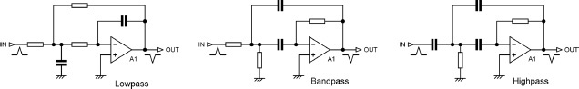
The multiple-feedback (MFB) filter is also called the Deliyannis filter; it is most familiar as a bandpass filter working at a modest Q, but the basic configuration can also be used to make lowpass and highpass filters. The variations are shown in Figure 10.1; the bandpass version is dealt with in more detail in Chapter 12.

Multiple-feedback (MFB) filters have the advantage that since they use shunt feedback, with a virtual earth at the inverting input, there is no common-mode voltage to cause distortion in the opamp. This is in contrast with the Sallen & Key filter, where the opamp is working as a voltage-follower, and so the full output signal voltage appears at the opamp inputs; it is the worst case for common-mode distortion. This potential problem is dealt with at length in Chapter 16, but it is worth pointing out here that if you use bipolar opamps such as the 5532 and relatively low source impedances, common-mode distortion is not likely to be a serious difficulty.

One awkward point that stands out is that the highpass MFB uses three capacitors rather than two, which is very unusual in a 2nd-order circuit. Since capacitors are more expensive than resistors, this is a definite drawback. The highpass MFB filter also seems to have some unhelpful performance issues, such as higher noise and distortion than the Sallen & Key equivalent. There is more on the noise and distortion performance of MFB filters in Chapter 11, but I’ll tell you now, I would not rush into highpass MFB filters.

Multiple-Feedback 2nd-Order Lowpass Filters

A practical version of an MFB lowpass filter is shown in Figure 10.2, designed for a Butterworth characteristic (Q = 0.7071) and a cutoff frequency of 1 kHz; the passband gain is unity. Note that if C1 is a preferred value, C2 will in general not be; the value of 104 nF shown here would in practice be approximated by 100 nF in parallel with 4n7. As usual the resistor values do not work out conveniently, but very close approximations to these values can be cheaply made up using 2xE24 parallel pairs of preferred values. MFB bandpass, highpass, and lowpass filters all inherently give a phase inversion. This is no problem if they are used in pairs in a 4th-order Linkwitz-Riley crossover, but otherwise could be inconvenient, in the worst case requiring another stage that does nothing but invert the signal to get it in-phase again.

It is worth pointing out that the MFB lowpass filter does not depend on a low opamp output impedance to maintain stopband attenuation at high frequencies, and so avoids the oh-no-it’s-coming-back-up-again behaviour of Sallen & Key lowpass filters. It is doubtful however if this is of much relevance to crossover applications.

Multiple-Feedback 2nd-Order Highpass Filters

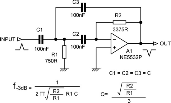
The multiple-feedback highpass filter is the multiple-feedback lowpass filter with the resistors and capacitors interchanged. A practical version of an MFB highpass filter is shown in Figure 10.3, once more designed for a Butterworth characteristic (Q = 0.7071), a cutoff frequency of 1 kHz, and unity passband gain.

This time we have three identical capacitors which can be conveniently chosen from the E6 series, dealing with the awkward resistor values in the usual way; as it happens, in this case R1 comes out as the E24 value of 750 Ω. There may be three capacitors, but this is still a 2nd-order circuit. Given the relatively high cost of capacitors compared with other components, this is not a particularly appealing configuration.

Multiple-Feedback 3rd-Order Filters

Filters of higher order using MFB stages can be made in the same way as for Sallen & Key stages; the appropriate cutoff frequencies and Q’s for each stage are taken from Chapter 7 and the stages placed in series, in a suitable order that minimises headroom restrictions due to gain peaking. Buffer amplifiers are used as required to make sure that 1st-order circuits are not loaded by succeeding stages.

As for Sallen & Key filters, these buffer amplifiers can be dispensed with if the loading effects are taken into account in the design; this does however make the process much more difficult and is likely to make component sensitivities worse. I have never used these filters myself, and I think caution should be the watchword. Clearly an amplifier is saved; however, you can also make both lowpass and highpass 3rd-order Sallen & Key filters in one stage and therefore using only one amplifier. Examples of 3rd-order Butterworth lowpass and highpass filters are given next, which can be scaled for different cutoff frequencies.

Multiple-Feedback 3rd-Order Lowpass Filters

A 3rd-order lowpass MFB filter can be made by placing an additional 1st-order lowpass circuit R4-C4 just before the 2nd-order MFB filter. In Figure 10.4 R4 = R1 = R2 = R3/2.

Multiple-Feedback 3rd-Order Highpass Filters

A 3rd-order highpass MFB filter can be made by placing an additional first-order highpass circuit C4-R4 just before the 2nd-order MFB filter. In Figure 10.5, C4 = C1 = C2 = 2C3. There is a clear temptation to make C3 the preferred value of 47 nF. If you do, the cutoff frequency and the later roll-off are unaffected, but the gain in the passband is increased from 0 dB to +0.54 dB; you can probably live with this. Although there are four capacitors, this is still a 3rd-order filter, in the same way that Figure 10.3 has three capacitors but is only a 2nd-order filter. Given the relatively high cost of capacitors, this is not an economic circuit.

Biquad Filters

Most biquad filters are composed of three amplifier stages in a loop. It is also possible to make biquads using just one amplifier with passive components around it, and they are unsurprisingly known as single-amplifier biquad (SAB) filters. Interest in SAB filters was high when the amplifiers were by a long way the most expensive parts in the circuit; that is no longer the case—it is now normally the capacitors which are the most expensive parts, unless for some reason you are using exotic opamps. SABs have their drawbacks and are not considered here.

Akerberg-Mossberg Lowpass Filter

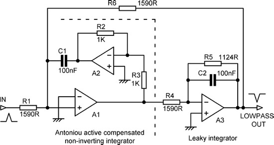
The Akerberg-Mossberg filter [2] uses three amplifiers. It is best suited to lowpass applications. It is a combination of an Antoniou active compensated non-inverting integrator (A1 and A2) and a leaky integrator (A3). The point of the Antoniou integrator [3] is that it does not invert, and so A3 can be a simple inverting stage, and that routing the negative feedback through A2 actively compensates for the finite bandwidth of A1, increasing their combined bandwidth. The inverted feedback via A2 means that the summing point (virtual earth) of the integrator is at the non-inverting input of A1, as in Figure 10.6, which shows an Akerberg-Mossberg 2nd-order Butterworth lowpass filter with a cutoff frequency of 1 kHz. It may look wrong in the diagram, but I assure you that’s how it’s supposed to be connected. A leaky integrator is an integrator with a resistance R5 placed across the capacitor C2.

The Akerberg-Mossberg filter is claimed to be superior to others in that it is very insensitive to amplifier shortcomings in gain and bandwidth. With modern opamps, this is not the big issue it used to be, but the configuration is also useful for generating higher Q’s than are practicable with the Sallen & Key or MFB configurations. Q’s of 400 or more are possible, if not obviously useful for crossover design. But … before you get too confident, read about the implementation problems I had.

Multiple opamp filters sometimes yield a useful signal at every opamp output, the classic case being the state-variable filter. This is not the case here; the output of A1 is a −6 dB/octave roll-off, which seems unlikely to be useful in crossover design. This point also shows +3 dB of gain in the passband, which is very likely to cause headroom problems. The output of A2 is the same as the output at A1 but phase inverted; also of little or no use to us. The lowpass signal at A3 output is phase inverted with respect to the input in the passband, which is likely to be inconvenient unless you are cascading two of them.

As usual it is best to choose the capacitor values and let the resistors come out as they may. The usual design process for a Butterworth characteristic with Q = 0.7071 is:

R2 and R3 have no link with the value of R; they just have to be equal.

These equations give the 1 kHz lowpass filter seen in Figure 10.6, and it works very nicely except for a couple of non-obvious snags. First, when designing a filter with more than one amplifier it really is essential to check every amplifier output to see if it has a higher signal level than the actual filter output. It is very necessary here; the A-M filter in Figure 10.6 has a gain of +3.2 dB in the passband at the A1 and A2 outputs, seriously degrading headroom (or signal/to noise, if you drop the nominal level by 3.2 dB to accommodate this gain). This is illustrated in Figure 10.7, showing measured results from the circuit of Figure 10.6; A1 has a higher output level than A3 and only falls at −6 dB/octave. So far as I am aware this is a standard Akerberg-Mossberg lowpass filter.

I decided to try and do something about this level problem. I reasoned that it would be best to leave the Antoniou integrator alone, as any modifications would mess up the active compensation process. That leaves leaky integrator A3. It occurred to me that if R4 was reduced by a factor of √2 (3 dB) and R6 increased by √2, the level at A1 and A3 outputs would be same, but the Antoniou integrator would not know that anything had changed. Since R5 has not been altered, C2 remains the same value as C1, and an awkward capacitor value is avoided; see Figure 10.8. This process works very nicely, and I believe it is a new finding; I therefore intend to call this the Akerberg-Mossberg-Self filter. OK?

The second snag proved less tractable. All was going very nicely until I attempted to measure the noise and distortion of the filter. A version using 5532 sections showed odd jumps in THD with frequency, and generally too much THD altogether. The cause seems to be some sort of complicated VHF instability in the ingenious Antoniou integrator. Before anyone asks, A1 and A2 were in the same dual package to get amplifier matching. A TL072 was tried for A1, A2, in the hope that its lower open-loop gain would fix the situation, but the results were much the same. An LM4562 was also tried in this position, but again the same problems appeared. I have some experience in taming recalcitrant circuitry, but there didn’t seem to be any way to fix this example. This was my first attempt at active compensation, and I am not impressed.

There the Akerberg-Mossberg situation rests for the present. Right now, if I needed to get a filter into production quickly, I wouldn’t touch it with my worst enemy’s bargepole.

The name is sometimes seen spelt “Ackerberg-Mossberg”, but “Akerberg-Mossberg” is the correct usage.

Akerberg-Mossberg Highpass Filters

The Akerberg-Mossberg is not much suited to making highpass filters. It can be done by replacing R1 with a third capacitor C3 connected to the inverting input of A3, as in Figure 10.9. There is now a bandpass response available at A1 and A2 outputs. A serious drawback is that the input is through C3 to a virtual ground, and the input impedance will be very low at high frequencies. Thus a 1 V input at 1 kHz gives input current of 628 uA, but at 20 kHz it is 12.5 mA. There are also likely to be stability issues with opamps driving large capacitive loads.

There are also three capacitors instead of two, adding to the cost. However, errors in the value of C3 do not affect the cutoff frequency or Q of the filter, just the gain, moving the response up or down without changing its shape. Depending on the application, this may mean that the accuracy of C3 can be relaxed compared with C1 and C2.

Overall, the highpass Akerberg-Mossberg filter is interesting but not recommended. I have therefore not given the detailed design process.

Tow-Thomas Biquad Lowpass and Bandpass Filter

This lowpass and bandpass biquad filter configuration was introduced by Tow [4] and Thomas [5], [6] and is sometimes called the Ring-of-Three circuit. It should not be confused with the Ring-of-Two circuit, which is a clever way of making a voltage reference [7] and nothing to do with active filters. There are other multi-amplifier biquad configurations, but if the term “biquad” is used without qualification it normally means the Tow-Thomas biquad. All biquads are inherently 2nd-order, because the response is controlled by quadratic equations, but they can be cascaded into higher-order filters in the same way as other 2nd-order filters.

The Tow-Thomas biquad has advantages over other types of active filter. The component sensitivities are low. The distortion performance is good because all three amplifiers are working in shunt-feedback mode, so there is no common-mode signal on the opamp inputs and therefore no common-mode distortion. This is very much in contrast to the Sallen & Key filter, which usually has the full signal voltage on the inputs. The TT biquad was built and measured (see Chapter 11) and proved very tractable and easy to apply. Unlike the Akerberg-Mossberg filter …

The Tow-Thomas biquad gives lowpass and bandpass responses simultaneously; this might allow for some elegant fill-driver crossovers (see Chapter 4) so long as the bandpass output has the correct Q. The bandpass output has −6 dB/octave skirts. The TT does not directly give a highpass output. Configurations that give all three responses directly are often called universal filters rather than biquads; the KHN state-variable filter is the best-known example and is dealt with later in this chapter. The TT biquad is sometimes confused with the KHN state-variable filter because it has three amplifiers and apparently two integrators, but in the TT A1 is actually a leaky integrator, due to the presence of R3, and not a pure integrator like A2; the filter operation is quite different.

Figure 10.10 shows a Tow-Thomas 2nd-order Butterworth lowpass filter designed to give 0 dB gain in the passband of the lowpass output at A2. The lowpass output from A2 is in phase with the input in the passband. The output from A3 is the same signal as at A2 but phase inverted, and it has to be said that having two lowpass outputs in anti-phase is rarely if ever useful in crossover design. The inverter is essential to the circuit operation, but as I have said elsewhere it irks me to have an opamp doing just a phase inversion; it hardly seems to be earning its keep.

The design process is:

Decide the passband gain A required.

(It is not essential to have C1 = C2, but it is obviously convenient and simplifies the design.)

Choose a convenient value for R2, such as 1 kΩ.

This however has deeper implications than mere convenience, which will be explained in a moment.

In any multi-amplifier filter, unity gain at one amplifier output can co-exist with more gain at the others, which will cause premature clipping internal to the filter. This needs to be checked for by simulation for each amplifier across the whole working frequency range. Here the output of A3 is clearly at the same level as A2, so no problem there. But … simulation shows a peak gain of +1.0 dB at the A1 bandpass output, which is not exactly disastrous but not ideal for maximum headroom; we can do better. The gain in the lowpass passband is always unity so long as R1 = R2.

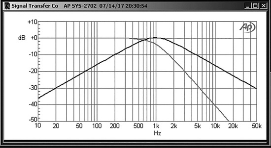
The initial choice of R2 = 1000 Ω gave us Figure 10.10. The gain at A1 output can be reduced by increasing the initial value of R2. So we try setting R2 = 1100 Ω and find that recalculating the values of R3 and R4 gives a peak gain at A1 output of only +0.2 dB, which we can ignore. R1 is now also set to R2 = 1100 Ω to maintain unity gain in the lowpass passband. R3 remains at the same value, since R2 does not appear in Equation 10.9, but R4 does change; see Figure 10.11. The frequency response of this circuit is shown in Figure 10.12. We will call it TT Version 1; see Table 10.3.

The full analysis equations for the Tow-Thomas biquad, including non-equal capacitors, are:

If C1 = C2 = C and R2 = R4 = R, which is also likely to be true in many cases, the analysis equations are much simplified:

One of the advantages of the Tow-Thomas biquad over Sallen & Key configurations is that it allows what is called orthogonal tuning. This means that the three parameters of frequency f₀, Q, and gain can be adjusted independently if it is done in the right order; thus:

1. Adjust R2 to get the required cutoff frequency f₀.
2. Adjust R3 to get the required Q. This will not affect the f₀ previously set.
3. Adjust R1 to get the desired passband gain A. This will not affect f₀ or Q.

As R1 is feeding into a virtual earth point, this is pretty obvious, unlike Step 2.

This will not be useful for production purposes, as presumably all parameters have been decided and fixed by the use of fixed resistors. It can however be very handy during crossover development work.

If the filter Q is greater than 0.7071 (1/√2), then gain peaking will occur at the lowpass output around the cutoff frequency. If we assume a Q of 1 is required, as is used to make up a two-stage 3rd-order Butterworth filter, then the peaking is +1.25 dB, which has a small effect on the headroom. We will call this TT Version 2, with the component values given in Table 10.3; they give 0 dB peak gain for the bandpass output, so there will be no headroom problems there. If you want to avoid any compromise on the headroom, the passband gain can be reduced as required by increasing the input resistor R1.

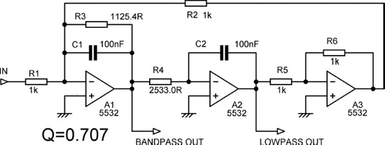
TT Version 3 is a TT example with a Q of 2.56, the highest Q required in a four-stage Butterworth 8th-order filter. If we try R2 = 1000 Ω we get R3 = 4074.4 Ω and R4 = 2533.0 Ω. SPICE simulation then shows us that the gain peaks at +8.2 dB at the lowpass output, which is what we expect with a Q that is relatively high by crossover standards; the passband gain is still unity. However, as with all multi-stage filters, we must check the levels at every amplifier output. The A3 output is an inverted version of A2 output, so there are no problems there. But … at A1 the bandpass output peaks at +12.1 dB at the cutoff frequency, and that is going to restrict headroom.

As we saw in the first example, the gain at A1 output can be reduced by increasing the initial value of R2; this leads to a lower value for R4, so less gain is required in the A1 stage to give the same output at A2. R1 is then increased in the same ratio as R2 to keep the lowpass passband gain at unity. This process is illustrated in Table 10.2, which shows how increasing the initial value of R2 affects the other components and the gain distribution in the filter. Note that R3 does not change, as the Q is not changing.

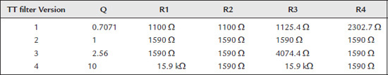
For crossover purposes R2 = 1590 Ω, giving equal peak gain at A1 and A2, gives probably the best noise/headroom compromise; we will call this TT Version 3. If for some reason you want near-unity gain at A1 output, you can see that R4 is getting too low; since it is driving a virtual earth, it is directly loading A1 output, and the distortion performance will suffer. In this case it would be better set C1 = C2 = 47 nF, which doubles the impedances. If then you set R1 = R2 = 8200 Ω, R3 emerges as 8668.9 Ω and R4 becomes 1398.4 Ω. R5 and R6 remain unaltered.

Suppose that for some reason you need a Q that is high by crossover standards; I’ll assume we want a lowpass with a Q of 10. This obviously gives some serious gain peaking—ten times or +20 dBu at the cutoff frequency. If it’s important to maintain full headroom at cutoff, then the only option is to reduce the passband gain by 20 dB, accepting there will be a noise penalty. This has been done in TT Version 4 in Table 10.3, so the gain at both lowpass and bandpass outputs is 0 dB at cutoff.

Table 10.3 summarises the component values for the versions of the Tow-Thomas biquad we have designed. In each case C1 and C2 are 100 nF and R5 and R6 are equal.

Tow-Thomas Biquad Notch and Allpass Responses

The basic Tow-Thomas biquad gives only bandpass and lowpass outputs. However, by suitably summing these outputs and also the input signal, notch, allpass, and highpass responses can be obtained, as in Figure 10.13.

You will have spotted that a little bit of tweaking has been done to some of the resistors. R7 had to be adjusted to get a convincingly deep notch, simulation showing −58 dB. R10 had to be adjusted to get a suitably flat allpass output, simulation showing it flat to within ±0.01 dB. R13 had to be adjusted to keep the highpass output falling with frequency at −12 dB/octave down to −80 dB at 10 Hz; without the correct value the slope lessens to −6 dB/octave within the audio band. You will note that all the resistors were tweaked to exactly the same value, indicating that the design of the basic Tow-Thomas biquad is off by a fraction; the gain to the output of A1 is clearly 0.2 dB high. This is the gain value we decided to live with in the previous section, but now that we are making derived outputs, it is a decided nuisance. Putting the tweaked resistors back to 1 kΩ and recalculating the biquad with a fractionally higher initial value for R2 would give a more elegant result, but since there is a better way to make a highpass Tow-Thomas, as described in the next section, and that is more likely to be useful in active crossover design than notches or allpass filters, I have not pursued that further at present.

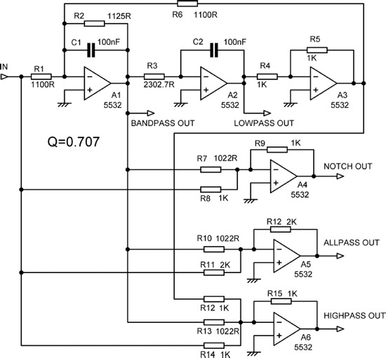
In all derived outputs of this sort the summing resistors have to be accurate, as notch depth, allpass flatness, and the highpass −12 dB/octave slope are all critically dependent on precision summing.

Tow-Thomas Biquad Highpass Filter

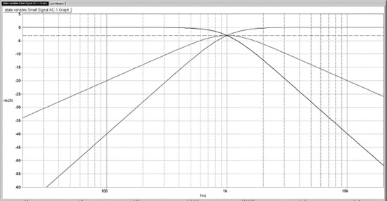
In the previous section we saw that deriving a highpass output from the standard Tow-Thomas biquad required four amplifiers and some critically accurate extra resistors. It is not an elegant solution, which is unfortunate, as active crossover design requires both lowpass and highpass filters. Mark Fortunato of Texas Instruments has reported a rearrangement of the Tow-Thomas configuration that gives a highpass output directly; [8] see Figure 10.14. The highpass output comes directly from A3. At A1 there is a bandpass output with−6 dB/octave skirts. At A2 there is a 1st-order roll-off with gain peaking just below the cutoff frequency; this is unlikely to be useful for anything.

As initially designed, R5 was set to 1 kΩ. For an input of 0 dB this gave a +2 dB peak at A2 output. It was decided that headroom was probably more desirable than the ultimate noise performance, so the circuit was recalculated with R5 set to 820R. This changes R2, and also R3 very slightly. R4 is unchanged, so this filter seems to have some of the orthogonal tuning features of the standard Tow-Thomas biquad. The alteration gives a gain peak at A2 of only +0.2 dB, which I think we can ignore. The level at A1 output now peaks at −5 dB, and there are no headroom issues there.

I have not derived the design equations for this filter. This is not as big a snag as you might think. Spreadsheets have facilities to set one quantity to a desired value by twiddling another; in Excel the feature is called Goalseek, and it is usually reliable, though I have known some equations to defeat it. This makes it fairly simple to work backwards from the analysis equations to get a design.

This is much sounder proposition for making an accurate TT highpass filter than the summation method; it uses one less amplifier, but perhaps more importantly, eliminates three precision resistors.

State-Variable Filters

State-variable filters (SVFs) give highpass, bandpass, and lowpass outputs simultaneously. In crossover applications the bandpass output is not likely to be used, except perhaps for filler-driver applications. The Tow-Thomas biquad configuration looks similar, but is only a lowpass and bandpass filter with no highpass output. SVF filters show good component value sensitivity and are very simple to design. They are called “state-variable” filters because in the most common 2nd-order version, they are made up of two integrators and an amplifier, and signals from all three stages are used for feedback (the output of each integrator and the output of the amplifier). These three variables completely define the state of the circuit. Higher-order state-variable filters have more integrators but also a feedback signal from each of them. The state-variable filter is often called a KHN filter in textbooks, after Kerwin, Huelsman, and Newcombe, who introduced the configuration. Like the Tow-Thomas biquad, the SVF is a tractable and easy-to-use filter.

A basic 2nd-order SVF is shown in Figure 10.16. The input is applied to the inverting input of amplifier A1. As shown it has unity gain in the passbands of the highpass and lowpass outputs, and a gain of −3 dB at the passband centre of the bandpass output. The highpass output is phase inverted in the passband, the bandpass output is in-phase in the centre of the passband, and the lowpass output is phase inverted in the passband. The presence of two integrators indicates that it is a 2nd-order filter. Higher-order state variable filters are perfectly possible; for example a 4th-order state-variable filter has four integrators; higher-order SVFs are dealt with later in this chapter.

The amplitude responses of the three outputs can be seen in Figure 10.17, where the −3 dB points of the high and lowpass filters coincide with the band centre of the bandpass output at 1 kHz. The Q is set at 0.7071 to give a Butterworth filter characteristic at the lowpass and highpass outputs, such as might be used in a 2nd-order crossover application. This low Q gives a very broad bandpass characteristic, with no peaking at the centre. The lowpass and highpass outputs both have an ultimate slope of 12 dB/octave, as we would expect from a 2nd-order filter, while the bandpass output has slopes of 6 dB/octave on each side of its peak. Since the cutoff frequencies of the highpass and lowpass filters are inherently the same, this is obviously a very convenient way to make a 2nd-order crossover in one handy stage. This does however mean that it is not possible to employ frequency offset between the highpass and lowpass filters.

The state-variable filter may look more complex than the Sallen & Key or the MFB filter, but it is in fact delightfully simple to design. Choose a resistor value R = R1 = R2 = R3 = R4, and choose a capacitor value C = C1 = C2.

The required centre frequency f is then used to calculate R6 and R7:

and Q is set by selecting an appropriate value for R5. For Butterworth it is 1.125 times the value of R.

To obtain other filter characteristics, it is necessary to set a different value of Q and use a frequency scaling factor to get the desired cutoff frequency, as we did with other forms of filter. So, to get a Bessel characteristic with a cutoff frequency of 1 kHz, R5 is set to 0.575 times R, and Equation 10.20 uses 1.273 times f as its input. The necessary values for the Q and scaling factor are given in Table 10.4

You will note that the lower the value of R5, the lower the Q; this is because the feedback path from the first integrator controls the damping of the circuit: the more feedback, the more damping.

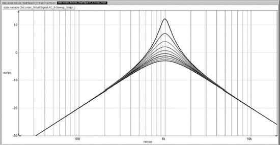
Q can also be altered by changing the value of R3. Figure 10.18 shows the effect on the bandpass output Q of stepping R3 from 1000 Ω down to 100 Ω; as R3 is reduced, the filter Q increases, because the damping feedback signal is being reduced. It increases more rapidly at lower values of R3. If a variable Q control is required, a reverse-log type gives an acceptable law. The higher the Q, the higher the passband gain at the peak, which is usually very inconvenient in crossover and equalisation work; in Figure 10.18 the maximum Q gives a gain of +12 dB. Changes in Q have a minimal effect on the skirts of the bandpass plot away from the peak.

An alternative approach is to apply the input to the non-inverting input of amplifier A1, as in Figure 10.19. Now, as R3 is reduced, the Q is increased as before, but simultaneously the input signal is attenuated to a greater extent, giving a constant gain at the bandpass peak, as illustrated in Figure 10.20. This method is sometimes called a constant-amplitude state-variable filter, though that condition only applies to the bandpass peak. It is particularly useful for implementing parametric equalisers; see Chapter 14. Changes in Q now do affect the skirts of the bandpass plot, and as before, the rate of change of Q accelerates as Q increases. The gain at the passband peak is set by the ratio of R1 and R5, and here is unity. Note that the phase relationships between input and outputs are in each case inverted with respect to that of Figure 10.16.

A notch output from a state-variable filter, with its centre at the same frequency as the bandpass output, can be obtained by the“1-bandpass” principle. The bandpass output is subtracted from the input signal by a fourth opamp. This is a relatively complicated way of making a notch filter, requiring precision resistors to get a good notch depth, and is not usually justified unless the ease of changing the centre frequency and Q which come with a state-variable filter is important. For fixed notches the Bainter filter is recommended, because its notch depth does not depend on the precise matching of resistors; see Chapter 12.

Variable-Frequency Filters: State-Variable 2nd Order

The number of gangs in a crossover frequency control can be halved by abandoning the use of separate filters and instead using state-variable filters that produce outputs for two paths simultaneously; this technology is widely if not universally used in variable-frequency crossovers. We saw earlier that a two-gang variable resistor controls the cutoff frequencies of both the lowpass and highpass outputs simultaneously.

Figure 10.21 shows a variable-frequency 2nd-order state-variable filter based on the design of Figure 10.19. The frequency-control method is slightly more sophisticated than just using the frequency pots as variable resistors, because it aims to reduce the effect of control mismatches. The variable resistors are now being used as potentiometers, so to a first approximation the effect of differing total track resistances will cancel out. To make this effective the loading on the potentiometer needs to be light relative to the track resistance, and you will observe that R6, R7 have been increased in value by ten times, while C1 and C2 have been reduced in value by ten times, to raise the impedances without altering the centre frequency range. This will of course have some consequences in terms of increased noise. Log controls can be used to get a suitable frequency calibration law. Altering the potentiometer setting alters the effective value of R6 and R7, and so the filter centre frequency. R8 and R9 are end-stop resistors to limit the frequency range at the lower end. Note that in this case the bandpass output of A2 is not used.

Variable-Frequency Filters: State-Variable 4th-Order

While the 2nd-order variable-frequency SVF works very nicely, 2nd-order crossovers are not exactly the most popular choice, because of their relatively shallow slopes and considerable band overlap. What is much more desirable is a variable-frequency 4th-order Linkwitz-Riley state-variable crossover; precisely this was provided by Dennis Bohn in 1983, [9] and this very clever implementation has seen extensive use in the crossover business. Figure 10.22 shows a 4th-order variable filter with a crossover frequency range from 210 Hz to 2.10 kHz. Note that there are now four integrators plus the summing/differencing stage, to which feedback from all four integrators is returned. As usual the capacitors have been made preferred values, letting the resistor values fall where they may.

Figure 10.23 shows the lowpass and highpass outputs from the 4th-order filter. The two outputs are both 6 dB down at the crossover frequency, as expected for a Linkwitz-Riley crossover, and the ultimate slopes are at 24 dB/octave. The design of the filter for various frequencies is not hard. It follows the same process as the 2nd-order SVF described earlier. Ignoring the variable resistors, and treating R8, R9, R10, and R11 as the total resistance feeding each integrator from the previous stage, the centre frequency f is then set by choosing R6 (= R7):

Note that the resistors around A1 have to be in the ratio shown for correct operation and to get the correct Q for a Linkwitz-Riley alignment. The required ratios are shown in brackets in Figure 10.22.

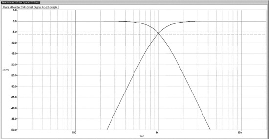
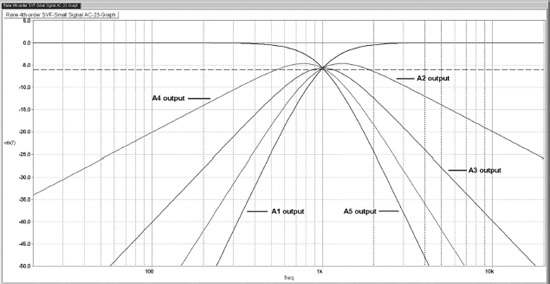
Figure 10.24 attempts to give some insight into how the filter works. The output from A1, the summing/differencing stage, is the highpass output, with an ultimate roll-off slope of 24 dB/octave below crossover as frequency decreases. The output of the first integrator A2 is the same but with a 6 dB/octave slope decreasing with frequency applied across the whole range, so the part of the response that was flat now slopes downward at 6 dB/octave slope with frequency, while the 24 dB/octave section has its slope reduced by 6 dB/octave to give 18 dB/octave. The second integrator A3 performs the same process again, so its output is a 4th-order bandpass response with skirt slopes of 12 dB/octave. The third integrator A4 does the same thing, its output having a 6 dB/octave slope in its low-frequency section, and a 18 dB/octave slope in its high-frequency section. The fourth integrator completes the process, and its output is the lowpass signal, with a flat low-frequency section and a 24 dB/octave roll-off above the crossover frequency. Note that all the plots in Figure 10.24 pass through the −6 dB point at the crossover frequency.

This 4th-order configuration could of course be adapted for fixed-frequency operation by removing the variable elements.

Variable-Frequency Filters: Other Orders of State-Variable

You may at this point be wondering what happened to 3rd-order state-variable filters; there appears to be no reason why these should not be constructed in exactly the same way, using three integrators plus a summing/differencing stage. In view of the lesser desirability of 3rd-order crossovers compared with 4th-order, I have chosen not to investigate these at this time. It is certainly possible to make 8th-order variable-frequency state-variable filter crossovers by using the same approach, as demonstrated by Dennis Bohn in 1988, [10] and so there is every reason to assume that 5th-, 6th-, and 7th-order versions could be implemented without great difficulty. Eighth-order crossovers are sometimes used in sound-reinforcement applications but seem unlikely to become popular in domestic hi-fi.

Other Filters

This chapter and the three preceding it by no means exhaust the filter types available. It is a fertile field for what Lord Rutherford would have called stamp-collecting. While I am not aware that the four filter configurations listed here have any special advantages for active crossover design, you may want to look them up. They are all multi-amplifier biquads.

• The Berka-Herpy biquad filter. [11]
• The Padukone-Mulawka-Ghausi (PMG) biquad filter. [12]
• The Mikhael-Bhattacharyya (MB) biquad filter. [13]
• The Natarajan biquad filter. [14] It is a modification of the standard Tow-Thomas biquad.

The first three use three amplifiers in the lowpass case, and the Natarajan lowpass uses four. The PMG and MB may or may not present technical challenges, but they certainly present spelling challenges and so are almost always referred to by their acronyms.

References

[1]Deliyannis, T., Yichuang Sun and J. K. Fidler “Continuous-Time Active Filter Design” CRC Press, 1999, pp. 127–134
[2]Akerberg, D., and Mossberg, K. “A Versatile Active RC Building Block with Inherent Compensation for the Finite Bandwidth of the Amplifier” IEEE Transactions on Circuits and System 21, pp. 75–78, 1974.
[3]Ananda Mohan, P. V. “VLSI Analog Filters, Active RC, OTA-C, and SC” Springer 2023, Section 2.2 ISBN: 978-0-8176-8357-3 (Print) 978-0-8176-8358-0 (Online)
[4]Tow, J. “Active RC Filters: A State-Space Realization” Proc IEEE, 56, 1968, pp. 1137–1139
[5]Thomas, L. C. “The Biquad: Part-I—Some Practical Design Considerations” IEEE Transactions on Circuit Theory CT18, pp. 350–361, 1971
[6]Thomas, L. C. “The Biquad: Part II—a Multipurpose Active Filtering System” IEEE Transactions on Circuit Theory CT-18(3), 1971, pp. 358–361,
[7]Hartley Jones, Martin “A Practical Introduction to Electronic Circuits” Third Edn, Cambridge University Press, 1995, pp. 226–227
[8]Fortunato, Mark “A New Filter Topology for Analog High-Pass Filters” Texas Instruments Analog Applications Journal SLYT299, 2008
[9]Bohn, D. A. “A Fourth-Order State Variable Filter for Linkwitz-Riley Active Filters” 74th AES Convention, October 1983, preprint 2011 (B-2)
[10]Bohn, D. A. “An 8th-Order State Variable Filter for Linkwitz-Riley Active Crossover Design” 85th AES Convention, November 1988, preprint 2697 (B-11)
[11]Chen, Wai-Kai (ed.) “The Circuits and Filters Handbook” Second Edition, CRC Press, 2003, pp. 2491–2492
[14]Natarajan, S. “Modified Tow-Thomas Biquads with Improved Active Sensitivity” Proceedings of the 30th Midwest Symposium on Circuits and Systems, August 17–18, 1987, held in Syracuse, New York