Chapter 15

Passive Components for Active Crossovers

In this chapter we will look at some passive component properties that are especially important in the design of small-signal audio equipment in general and active crossovers in particular. All passive components differ from the ideal mathematical models—resistors have series inductance, capacitors have series resistance, and so on. There are also well-known issues with the accuracy of the component value and the way that the value changes with temperature. What is less publicised is that some can show significant non-linearity.

It is most unwise to assume that all the distortion in an electronic circuit will arise from the active devices. This is pretty clearly not true if transformers or other inductors are in the audio path, but it is also a very unsafe assumption if the only passive components you are using are resistors and capacitors. I recall that I was horrified when I first began designing active filters; the distortion from the polyester capacitors completely obliterated the quite low THD from the discrete transistor unity-gain buffers I was using. More on this problem later.

Component Values

Active filters are the basic building blocks of electronic crossovers, and their proper operation depends on having accurate ratios between resistors and capacitors. Setting these up is complicated by the fact that capacitors are available in a much more limited range of values than resistors, often restricted to the E6 series, which runs 10, 15, 22, 33, 47, 68. Fortunately resistors are widely available in the E24 series (24 values per decade) and the E96 series (96 values per decade). There is also the E192 series (you guessed it, 192 values per decade), but this is less freely available. Using the E96 or E192 series means you have to keep a lot of different resistor values in stock, and when non-standard values are required it is usually more convenient to use a series or parallel combination of two E24 resistors. More on this later, too.

It is common in USA publications to see something like: “Resistor values have been rounded to the nearest 1% value”, which usually means the E96 series has been used. The value series from E3 to E96 is given in Appendix 5.

Resistors

In the past there have been many types of resistor, including some interesting ones consisting of jars of liquid, but only a few kinds are likely to be met with now. These are usually classified by the kind of material used in the resistive element, as this has the most important influence on the fine details of performance. The major materials and types are shown in Table 15.1.

These values are illustrative only, and it would be easy to find exceptions. As always, the official data sheet for the component you have chosen is the essential reference. The voltage coefficient is a measure of linearity (lower is better), and its sinister significance is explained later.

It should be said that you are most unlikely to come across carbon composition resistors in modern signal circuitry, but they frequently appear in vintage valve equipment, so they are included here. They also live on in specialised applications such as switch-mode snubbing circuits, where their ability to absorb a high peak power in a mass of material rather than a thin film is very useful.

Carbon film resistors are currently still sometimes used in low-end consumer equipment but elsewhere have been supplanted by the other three types. Note from Table 15.1 that they have a significant voltage coefficient.

Metal film resistors are now the usual choice when any degree of precision or stability is required. These have no non-linearity problems at normal signal levels. The voltage coefficient is usually negligible.

Metal oxide resistors are more problematic. Cermet resistors and resistor packages are metal oxide and are made of the same material as thick-film SM resistors. Thick-film resistors can show significant non-linearity at opamp-type signal levels and should be kept out of high-quality signal paths.

Wirewound resistors are indispensable when serious power needs to be handled. The average wirewound resistor can withstand very large amounts of pulse power for short periods, but in this litigious age component manufacturers are often very reluctant to publish specifications on this capability, and endurance tests have to be done at the design stage; if this part of the system is built first, then it will be tested as development proceeds. The voltage coefficient is usually negligible.

Resistors for general PCB use come in both through-hole and surface-mount types. Through-hole (TH) resistors can be any of the types in Table 15.1; surface-mount (SM) resistors are always either metal film or metal oxide. There are also many specialised types; for example, high-power wirewound resistors are often constructed inside a metal case that can be bolted down to a heatsink.

Through-Hole Resistors

These are too familiar to require much description; they are available in all the materials mentioned earlier: carbon film, metal film, metal oxide, and wirewound. There are a few other sorts, such as metal foil, but they are restricted to specialised applications. Conventional through-hole resistors are now almost always 250 mW 1% metal film. Carbon film used to be the standard resistor material, with the expensive metal film resistors reserved for critical places in circuitry where low tempco and an absence of excess noise were really important, but as metal film got cheaper, so it took over many applications.

TH resistors have the advantage that their power and voltage rating greatly exceed those of surface-mount versions. They also have a very low voltage coefficient, which for our purposes is of the first importance. On the downside, the spiral construction of the resistance element means they have much greater parasitic inductance; this is not a problem in audio work.

Surface-Mount Resistors

Surface-mount resistors come in two main formats, the common chip type and the rarer (and much more expensive) MELF format.

Chip surface-mount (SM) resistors come in a flat tombstone format, which varies over a wide size range; see Table 15.2.

MELF surface-mount resistors have a cylindrical body with metal endcaps, the resistive element is metal film, and the linearity is therefore as good as conventional resistors, with a voltage coefficient of less than 1 ppm. MELF is apparently an acronym for “Metal ELectrode Face-bonded” though most people I know call them “Metal Ended Little Fellows” or something quite close to that.

Surface-mount resistors may have thin-film or thick-film resistive elements. The latter are cheaper and so more often encountered, but the price differential has been falling in recent years. Both thin-film and thick-film SM resistors use laser trimming to make fine adjustments of resistance value during the manufacturing process. There are important differences in their behaviour.

Thin-film (metal film) SM resistors use a nickel-chromium (Ni-Cr) film as the resistance material. A very thin Ni-Cr film of less than 1 um thickness is deposited on the aluminium oxide substrate by sputtering under vacuum. Ni-Cr is then applied onto the substrate as conducting electrodes. The use of a metal film as the resistance material allows thin-film resistors to provide a very low temperature coefficient, much lower current noise and vanishingly small non-linearity. Thin-film resistors need only low laser power for trimming (one-third of that required for thick-film resistors) and contain no glass-based material. This prevents possible micro-cracking during laser trimming and maintains the stability of the thin-film resistor types.

Thick-film resistors normally use ruthenium oxide (RuO2) as the resistance material, mixed with glass-based material to form a paste for printing on the substrate. The thickness of the printing material is usually 12 um. The heat generated during laser trimming can cause micro-cracks on a thick-film resistor containing glass-based materials, which can adversely affect stability. Palladium/silver (PdAg) is used for the electrodes.

The most important thing about thick-film surface-mount resistors from our point of view is that they do not obey Ohm’s law very well. This often comes as a shock to people who are used to TH resistors, which have been the highly linear metal film type for many years. They have much higher voltage coefficients than TH resistors, at between 30 and 100 ppm. The non-linearity is symmetrical about zero voltage and so gives rise to third-harmonic distortion. Some SM resistor manufacturers do not specify voltage coefficient, which usually means it can vary disturbingly between different batches and different values of the same component, and this can have dire results on the repeatability of design performance.

Chip-type surface-mount resistors come in standard formats with names based on size, such as 1206, 0805, 0603, and 0402. For example, 0805, which used to be something like the “standard” size, is 0.08 inches by 0.05 inches; see Table 15.2. The smaller 0603 is now more common. Both 0805 and 0603 can be placed manually if you have a steady hand and a good magnifying glass.

The 0402 size is so small that the resistors look rather like grains of pepper; manual placing is not really feasible. They are only used in equipment where small size is critical, such as mobile phones. They have very restricted voltage and power ratings, typically 50 V and 100 mW. The voltage rating of TH resistors can usually be ignored, as power dissipation is almost always the limiting factor, but with SM resistors it must be kept firmly in mind.

Recently, even smaller surface-mount resistors have been introduced; for example several vendors offer 0201, and Panasonic and Yageo offer 01005 resistors. The latter are truly tiny, being about 0.4 mm long; a thousand of them weigh less than a twentieth of a gram. They are intended for mobile phones, palmtops, and hearing aids; a full range of values is available from 10 Ω to 1 MΩ (jumper inclusive). Hand placing is really not an option.

Surface-mount resistors have a limited power-dissipation capability compared with their through-hole cousins, because of their small physical size. SM voltage ratings are also restricted, for the same reason. It is therefore sometimes necessary to use two SM resistors in series or parallel to meet these demands, as this is usually more economic than hand-fitting a through-hole component of adequate rating. If the voltage rating is the issue, then the SM resistors will obviously have to be connected in series to gain any benefit.

Resistors: Values and Tolerances

Resistors come in a rich variety of values compared with other components such as capacitors, and this gives a much needed flexibility to crossover design and active filter design generally.

Active filters very often require both precise resistor values and precise resistor ratios. When designing circuit blocks such as Sallen & Key highpass filters, where resistor ratios of exactly two are required, it is useful to keep in mind the options in the E24 series, as in Table 15.3, and the E96 series, as in Tables 15.4 to 15.7. The E24 series offers six options for a ratio of two, while the E96 series offers 16. In both cases the 1:2 pairs are closely spaced at the bottom of the decade, and this will have to be taken into account when choosing capacitor values.

Other resistor ratios are less commonly used, but it is useful to be aware of them. In the E24 series there are four pairs of values in the ratio 1:3, two pairs in the ratio 1:4, and six pairs in the ratio 1:5; see Tables 15.5 to 15.7. In the E96 series there are no pairs in the ratio 1:3 or 1:4. This may sound paradoxical, but it is simply because the E96 series does not include many values from the E24 series. E12 is a subset of E24, but E24 is not a subset of E96. This less-than-obvious fact needs to be remembered when you are selecting resistors.

This information is also summarised in Appendix 5.

The standard tolerance for TH resistors is ±1%. In the direction of increasing accuracy, the next popular tolerance is ±0.1%; in the E24 series they cost between 10 and 15 times as much as the 1% parts but nowadays are freely available from the usual component distributors and are a good option when real precision is required in a few places in a crossover.

In many cases you will aim to use a capacitor value or values in the relatively sparse E6 series, and this will almost invariably result in non-standard resistor values. These are easily obtained by putting two or more resistors in series or parallel, and multiple resistors will be much cheaper than multiple capacitors. There are other advantages to this, as I shall now explain.

Improving Accuracy With Multiple Components: Gaussian Distribution

Using two or more resistors to make up a desired value has a valuable hidden benefit. If it is done correctly it will actually increase the average accuracy of the total resistance value so it is better than the tolerance of the individual resistors; this may sound paradoxical, but it is simply an expression of the fact that random errors tend to cancel out if you have a number of them. This works for any parameter that is subject to random variations, but for the time being we will focus on the concrete example of multiple resistors.

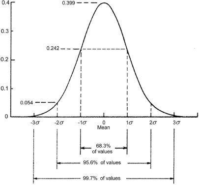
Resistor values are usually subject to a Gaussian distribution, also called a normal distribution. It has a familiar peaked shape, not unlike a resonance curve, showing that the majority of the values lie near the central mean and that they get rarer the further away from the mean you look. This is a very common distribution in statistics, cropping up wherever there are many independent things going on that all affect the value of a given component. The distribution is defined by its mean and its standard deviation, which is the square root of the sum of the squares of the distances from the mean—the RMS-sum, in other words. Sigma (σ) is the standard symbol for standard deviation. A Gaussian distribution will have 68.3% of its values within ±1 σ, 95.4% within ±2 σ, 99.7% within ±3 σ, and 99.9% within ±4 σ. This is illustrated in Figure 15.1, where the x-axis is calibrated in numbers of standard deviations on either side of the central mean value.

If we put two equal-value resistors in series, or in parallel, the total value has a narrower distribution than that of the original components. The standard deviation of summed components is the sum of the squares of the individual standard deviations, as shown in Equation 15.1; σsum is the overall standard deviation, and σ1 and σ2 are the standard deviations of the two resistors in series.

Thus if we have four 100 Ω 1% resistors in series, the standard deviation of the total resistance increases only by the square root of 4, that is 2 times, while the total resistance has increased by 4 times; thus we have inexpensively made an otherwise costly 0.5% close-tolerance 400 Ω resistor. There is a happy analogue here with the use of multiple amplifiers to reduce electrical noise; we are using essentially the same technique to reduce “statistical noise”. Note that this equation (Equation 15.1) only applies to resistors in series and cannot be used when resistors are connected in parallel to obtain a desired value. The improvement in accuracy nonetheless works in the same way.

You may object that putting four 1% resistors in series means that the worst-case errors can be four times as great. This obviously true—if all the components are 1% low, or 1% high, the total error will be 4%. But the probability of this occurring is actually very, very small indeed. The more resistors you combine, the more the values cluster together in the centre of the range.

Perhaps you are not wholly satisfied that this apparently magical improvement in average accuracy is genuine. I could reproduce here the standard statistical mathematics, but it is not very exciting and can be easily found in the standard textbooks. I have found that showing the process actually at work on a spreadsheet makes a much more convincing demonstration.

In Excel, the standard random numbers with a uniform distribution are generated by the function RAND(), but random numbers with a Gaussian distribution and specified mean and standard deviation can be generated by the function NORMINV(). Let us assume we want to make an accurate 20 kΩ resistance. We can simulate the use of a single 1% tolerance resistor by generating a column of Gaussian random numbers with a mean of 20 and a standard deviation of 0.2; we need to use a lot of numbers to smooth out the statistical fluctuations, so we generate 400 of them. As a check we calculate the mean and standard deviation of our 400 random numbers using the AVERAGE() and STDEV() functions. The results will be very close to 20 and 0.2, but not identical, and will change every time we hit the F9 recalculate key, as this generates a new set of random numbers. The results of five recalculations are shown in Table 15.8, demonstrating that 400 numbers are enough to get us quite close to our targets.

To simulate the series combination of two 10 kΩ resistors of 1% tolerance we generate two columns of 400 Gaussian random numbers with a mean of 10 and a standard deviation of 0.1. We then set up a third column which is the sum of the two random numbers on the same row, and if we calculate the mean and standard deviation of that using AVERAGE() and STDEV() again, we find that the mean is still very close to 20, but the standard deviation is reduced on average by the expected factor of √2. The result of five trials is shown in Table 15.9. Repeating this experiment with two 40 kΩ resistors in parallel gives the same results.

If we repeat this experiment by making our 20 kΩ resistance from a series combination of four 5 kΩ resistors of 1% tolerance, we have to generate four columns of 400 Gaussian random numbers with a mean of 5 and a standard deviation of 0.05. We sum the four numbers on the same row to get a fifth column and calculate the mean and standard deviation of that. The result of five trials is shown in Table 15.10.The mean is very close to 20, but the standard deviation is now reduced on average by a factor of √4, which is 2.

I think this demonstrates quite convincingly that the spread of values is reduced by a factor equal to the square root of the number of the components used. The principle works equally well for capacitors or indeed any quantity with a Gaussian distribution of values. The downside is the fact that the improvement depends on the square root of the number of equal-value components used, which means that big improvements require a lot of parts and the method quickly gets unwieldy. Table 15.11 demonstrates how this works; the rate of improvement slows down noticeably as the number of parts increases. The largest number of components I have ever used in this way for a production design is five. Constructing a 0.1% resistance from 1% resistors would require a hundred of them and would not normally be considered a practical proposition, due to the PCB area and assembly time required.

The spreadsheet experiment is easy to do, though it does involve a bit of copy-and-paste to set up 400 rows of calculation. It takes only about a second to recalculate on my PC, which is by no stretch of the imagination state of the art.

You may be wondering what happens if the series resistors used are not equal. If you are in search of a particular value, the method that gives the best resolution is to use one large resistor value and one small one to make up the total, as this gives a very large number of possible combinations. However, the accuracy of the final value is essentially no better than that of the large resistor. Two equal resistors, as we have just demonstrated, give a √2 improvement in accuracy, and near-equal resistors give almost as much, but the number of combinations is very limited, and you may not be able to get very near the value you want. The question is, how much improvement in accuracy can we get with resistors that are some way from equal, such as one resistor being twice the size of the other?

The mathematical answer is very simple; even when the resistor values are not equal, the overall standard deviation is still the RMS-sum of the standard deviations of the two resistors, as shown in Equation 15.1; σ1 and σ2 are the standard deviations of the two resistors in series. Note that this equation is only correct if there is no correlation between the two values whose standard deviations we are adding; this is true for two separate resistors but would not hold for two film resistors fabricated on the same substrate.

Since both resistors have the same percentage tolerance, the larger of the two has the greater standard deviation and dominates the total result. The minimum total deviation is thus achieved with equal resistor values. Table 15.12 shows how this works, and it is clear that using two resistors in the ratio 2:1 or 3:1 still gives a worthwhile improvement in average accuracy.

The entries for 19.5k +500 and 19.9k +100 demonstrate that when one large resistor value and one small are used to get a particular value, its accuracy is very little better than that of the large resistor alone.

Resistor Value Distributions

At this point you may be complaining that this will only work if the resistor values have a Gaussian (also known as normal) distribution with the familiar peak around the mean (average) value. Actually, it is a happy fact this effect does not assume that the component values have a normal (Gaussian) distribution, as we shall see in a moment. An excellent account of how to handle statistical variations to enhance accuracy is in [1]. This deals with the addition of mechanical tolerances in optical instruments, but the principles are just the same.

Also we have assumed that the mean is absolutely accurate. This is actually completely reasonable because controlling the mean value emerging from a manufacturing process is usually easy compared with controlling all the variables that lead to a spread in values. In the examples given next, it is plain that the mean is very well controlled, and the spread is pretty much under control as well.

You sometimes hear that this sort of thing is inherently flawed, because, for example, 1% resistors are selected from production runs of 5% resistors. If you were using the 5% resistors, then you would find there was a hole in the middle of the distribution; if you were trying to select 1% resistors from them, you would be in for a very frustrating time, as they have already been selected out, and you wouldn’t find a single one. If instead you were using the 1% components obtained by selection from the 5% population, you would find that the distribution would be much flatter than Gaussian and the accuracy improvement obtained by combining them would be reduced, although there would still be a definite improvement.

However, don’t worry. In general this is not the way that components are manufactured nowadays, though it may have been so in the past. A rare contemporary exception is the manufacture of carbon composition resistors, [2] where making accurate values is difficult, and selection from production runs, typically with a 10% tolerance, is the only practical way to get more accurate values. Carbon composition resistors have no place in audio circuitry because of their large temperature and voltage coefficients and high excess noise, but they live on in specialised applications such as switch-mode snubbing circuits, where their ability to absorb high peak power in bulk material rather than a thin film is useful, and in RF circuitry where the inductance of spiral-format film resistors is unacceptable.

So, having laid that fear to rest, what is the actual distribution of resistor values like? It is not easy to find out, as manufacturers are not very forthcoming with this sort of information, and measuring thousands of resistors with an accurate DVM is not a pastime that appeals to all of us. Any nugget of information in this area is therefore very welcome; Hugo Kroeze [3] reported the result of measuring 211 metal film resistors from the same batch with a nominal value of 10 kΩ and1% tolerance. He concluded that:

1. The mean value was 9.995 k Ω (0.05% low).
2. The standard deviation was about 10 Ω, i.e. only 0.1%. This spread in value is surprisingly small (the resistors were all from the same batch, and the spread across batches widely separated in manufacture date might have been less impressive).
3. All the resistors were within the 1% tolerance range.
4. The distribution appeared to be Gaussian, with no evidence that it was a subset from a larger distribution.

I have added my own modest contribution of data to what we know. I measured 100 ordinary metal film 1kΩ resistors of 1% tolerance from Yageo, a reputable Chinese manufacturer, and very tedious it was too. If you think you can achieve some sort of Zen ecstasy by repeatedly measuring resistors, I can assure you it did not happen to me. I used a recently-calibrated 4.5 digit multimeter.

1. The mean value was 997.66 Ohms (0.23% low).
2. The standard deviation was 2.10 Ohms, i.e. 0.21%.
3. All resistors were within the 1% tolerance range. All but one was within 0.5%, with the outlier at 0.7%.
4. The distribution appeared to be Gaussian, with no evidence that it was a subset from a larger distribution.

These results are not as good as those obtained by Hugo Kroeze but reassuringly demonstrate that these ordinary commercial resistors were well within their specification, and using multiple parts to increase nominal accuracy should work well.

Now these are only two reports, and it would be nice to have more confirmation, but there seems to be no reason to doubt that the distribution of resistance values is Gaussian, though the range of standard deviations you are likely to meet remains enigmatic. Whenever I have attempted this kind of statistical improvement in accuracy, I have always found that the expected benefit really does appear in practice.

Improving Accuracy With Multiple Components: Uniform Distribution

As I mentioned earlier, improving average accuracy by combining resistors does not depend on the resistance value having a Gaussian distribution. Even a batch of resistors with a uniform distribution gives better accuracy when two of them are combined. A uniform distribution of component values may not be likely, but the result of combining two or more of them is highly instructive, so stick with me for a bit.

Figure 15.2a shows a uniform distribution that cuts off abruptly at the limits L and−L and represents 10 kΩ resistors of 1% tolerance. We will assume again that we want to make a more accurate 20 kΩ resistance. If we put two of the uniform-distribution 10 kΩ resistors in series, we get not another uniform distribution, but the triangular distribution shown in Figure 15.2b. This shows that the total resistance values are already starting to cluster in the centre; it is possible to have the extreme values of 19.8 kΩ and 20.2 kΩ, but it is very unlikely.

Figure 15.2c shows what happens if we use more resistors to make the final value; when four are used, the distribution is already beginning to look like a Gaussian distribution, and as we increase the number of components to eight and then 16, the resemblance becomes very close.

Uniform distributions have a standard deviation just as Gaussian ones do. It is calculated from the limits L and−Las in Equation 15.2. Likewise, the standard deviation of a triangular distribution can be calculated from its limits L and −L, as in Equation 15.3.

Applying Equation 15.2 to the uniformly-distributed 10 kΩ 1% resistors in Figure 15.2a, we get a standard deviation of 0.0577. Applying Equation 15.3 to the triangular distribution of 20 kΩ resistance values in Figure 15.2b, we get 0.0816. The mean value has doubled, but the standard deviation has less than doubled, so we get an improvement in average accuracy; the ratio is √2, just as it was for two resistors with a Gaussian distribution. This is also easy to demonstrate with the spreadsheet method described earlier.

Obtaining Arbitrary Resistance Values

If you are making up a particular resistance value, the best resolution is obtained by using one large resistor value and one small one to make up the total, so for example 3100 Ω would be made up of 3000 Ω and 100 Ω; this is what you might call the asymmetrical solution. On the other hand, if it is possible to make up the required value with two resistors of roughly the same value, there is an advantage in terms of increased precision, for the statistical reasons described previously. In the optimal case, where the two resistors are equal, the average accuracy is improved by √2, but resistors in the ratio 2:1 or 3:1 still give a useful improvement.

The best procedure is therefore to determine at the beginning how accurate the resistor value needs to be, start with two near-equal resistor values, and if no combination can be found within our error window, we try values that are more and more unequal until we get a satisfactory result. As an example, we will assume that we are using E24 values, and our calculations show that 2090 Ω is the exact value required. The closest we can get with near-equal resistors in series is 1000 Ω + 1100 Ω = 2100 Ω, an error of 0.48%, which you may well be able to live with. If not, we try again using near-equal resistors in parallel, and we come up with 4300 Ω in parallel with 3900 Ω = 2045 Ω; this is in error by −2.2%, which is rather less appealing. Clearly the series option comes up with the closer answer in this case, but if 2100 Ω is not close enough, one option is to abandon completely the “near-equal” constraint and go for one large value and one small value. The obvious answer is 2000 Ω + 91 Ω = 2091 Ω, which is an error of only +0.048%, small enough to be utterly lost in other component tolerances. However, there is no improvement in precision. As we saw in Table 15.12, intermediate conditions between “near equal” and “one large and one small” will give intermediate improvements in precision.

The equivalent asymmetrical parallel-combination best approach is 2200 Ω in parallel with 43 k = 2092.9 Ω, which has an error of +0.14%, and so the series solution is in this case the better one.

A step-by step example of choosing parallel resistor combinations for the best possible increased precision while achieving a result within a specified percentage error window is given in Chapter 23, where a complete active crossover is designed.

Trying out the various resistor combinations on a hand calculator rapidly becomes life-threateningly tedious, even on my much-prized Casio FX-19 scientific calculator, now more than 30 years old but still working beautifully. [4] A spreadsheet is somewhat quicker once you’ve set it up, but the best answer is clearly some software that automatically comes up with the best answers. One example is resistor combination calculator utility called “ResCalc” by Mark Lovell and Morgan Jones, [5] which is superior to most as it allows mixed E24 and E96 series, but like all the other resistor-calculator applications I have seen, it does not appear to prioritise near-equal values to minimise tolerance errors.

A closer approach to the desired value while keeping the values near equal is possible by using combinations of three resistors rather than two. The cost is still low because resistors are cheap, but seeking out the best combination is an unwieldy process. By the time this book appears I hope to have a Javascript solution on my website. [6]

All of the statistical features described here apply to capacitors as well but are harder to apply because capacitors come in sparse value series, and it is also much more expensive to use multiple parts to obtain an arbitrary value. It is worth going to a good deal of trouble to come up with a circuit design that uses only standard capacitor values; the resistors will then almost certainly be all non-standard values, but this is easier and cheaper to deal with. A good example of the use of multiple parallel capacitors, both to improve accuracy and to make up values larger than those available, is the Signal Transfer RIAA preamplifier; [7] [8] see also the end of this book. This design is noted for giving very accurate RIAA equalisation at a reasonable cost. There are two capacitances required in the RIAA network, one being made up of four polystyrene capacitors in parallel and the other of five polystyrene capacitors in parallel. This also allows non-standard capacitance values to be used.

Other Resistor Combinations

So far we have looked at serial and parallel combinations of components to make up one value, as in Figure 15.3a and 15.3b. Other important combinations are the resistive divider at Figure 15.5c, which is frequently used as the negative feedback network for non-inverting amplifiers. A two-output divider is shown at Figure 15.3d and a three-output divider at Figure 15.3e. Another important configuration is the inverting amplifier at Figure 15.5f, where the gain is set by the ratio R2/R1. All resistors are assumed to have the same tolerance about an exact mean value.

I suggest it is not obvious whether the divider ratio of Figure 15.5c, which is R2/(R1 + R2), will be more or less accurate than the resistor tolerance, even in the simple case with R1 = R2 giving a divider ratio of 0.5. However, the Monte Carlo method shows that in this case partial cancellation of errors still occurs, and the division ratio is more accurate by a factor of √2.

This factor depends on the divider ratio, as a simple physical argument shows:

• If the top resistor R1 is zero, then the divider ratio is obviously one with complete accuracy, the bottom resistor value is irrelevant, and the output voltage tolerance is zero.
• If the bottom resistor R2 is zero, there is no output and accuracy is meaningless, but if instead R2 is very small compared with R1, then R1 completely determines the current through R2, and R2 turns this into the output voltage. Therefore the tolerances of R1 and R2 act independently, and so the combined output voltage tolerance is worse by a factor of √2.

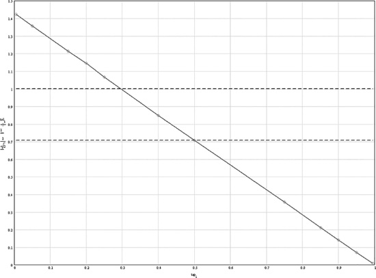
Some more Monte Carlo work, with 8000 trials per data point, revealed that there is a linear relationship between accuracy and the “tap position” of the output between R1 and R2, as shown in Figure 15.4. Plotting against division ratio would not give a straight line. With R1 = R2 the tap is at 50%, and accuracy improved by a factor of √2, as noted earlier. With a tap at about 30% (R1 = 7 kΩ, R2 = 3 kΩ) the accuracy is the same as the resistors used. This assessment is not applicable to potentiometers, as the two sections of the pot are not uncorrelated in value—they are highly correlated.

The two-tap divider (Figure 15.3d) and three-tap divider(Figure 15.3e) were also given a Monte Carlo work-out, though only for equal resistors. The two-tap divider has an accuracy factor of 0.404 at OUT 1 and 0.809 at OUT 2. These numbers are very close to √2/(2√3) and √2/(√3) respectively. The three-tap divider has an accuracy factor of 0.289 at OUT 1, of 0.500 at OUT 2, and of 0.864 at OUT 3. The middle figure is clearly 1/2 (twice as many resistors as a one-tap divider, so √2 times more accurate), while the first and last numbers are very close to √3/6 and √3/2 respectively. It would be helpful if someone could prove analytically that the factors proposed are actually correct.

For the inverting amplifier of Figure 15.3f, the values of R1 and R2 are completely uncorrelated, and so the accuracy of the gain is always √2 worse than the tolerance of each resistor, assuming the tolerances are equal. The nominal resistor values have no effect on this. We therefore have the interesting situation that a non-inverting amplifier will always be equally or more accurate in its gain than an inverting amplifier. So far as I know this is a new result. Maybe it will be useful.

Resistor Noise: Johnson and Excess Noise

All resistors, no matter what their method of construction, generate Johnson noise. This is white noise, which has equal power in equal absolute bandwidth, i.e. with the bandwidth measured in Hz, not octaves. There is the same noise power between 100 and 200 Hz as there is between 1100 and 1200 Hz. The level of Johnson noise that a resistor generates is determined solely by its resistance value, the absolute temperature (in degrees Kelvin), and the bandwidth over which the noise is being measured. For our purposes the temperature is 25 °C and the bandwidth is 22 kHz, so the resistance is really the only variable. The level of Johnson noise is based on fundamental physics and is not subject to modification, negotiation, or any sort of rule-bending … however, you might want to look up “load synthesis”, in which a high-value resistor is made to act like a low-value resistor but still having the low Johnson current noise of the high-value resistor. [9] Sometimes Johnson noise from resistors places the limit on how quiet a circuit can be, though more often the noise from the active devices is dominant. It is a constant refrain in this book that resistor values should be kept as low as possible, without introducing distortion by overloading the circuitry, in order to minimise the Johnson noise contribution and the effects of opamp current noise.

The rms amplitude of Johnson noise is calculated from the classic equation:

Where:

vn is the rms noise voltage	T is absolute temperature in °K	B is the bandwidth in Hz
k is Boltzmann’s constant	R is the resistance in Ohms

The thing to be careful with here is to use Boltzmann’s constant (1.380662 × 10⁻²³), and NOT the Stefan-Boltzmann constant (5.67 10⁻⁰⁸), which relates to black-body radiation, has nothing to do with resistors, and will give some impressively wrong answers. The voltage noise is often left in its squared form for ease of RMS-summing with other noise sources.

The noise voltage is inseparable from the resistance, so the equivalent circuit is of a voltage source in series with the resistance present. Johnson noise is usually represented as a voltage, but it can also be treated as a Johnson noise current, by means of the Thevenin-Norton transformation, [10] which gives the alternative equivalent circuit of a current source in shunt with the resistance. The equation for the noise current is simply the Johnson voltage divided by the value of the resistor it comes from:

Excess resistor noise refers to the fact that some resistors, with a constant voltage drop across them, generate extra noise in addition to their inherent Johnson noise. This is a very variable quantity, but is essentially proportional to the DC voltage across the component; the specification is therefore in the form of a “noise index” such as “1 uV/V”. The uV/V parameter increases with increasing resistor value and decreases with increasing resistor size or power dissipation capacity. Excess noise has a 1/f frequency distribution. It is usually only of interest if you are using carbon or thick-film resistors—metal film and wirewound types should have little or no excess noise. A rough guide to the likely range for excess noise specs is given in Table 15.13

One of the great benefits of opamp circuitry is that it allows simple dual-rail operation, and so it is noticeably free of resistors with large DC voltages across them; the offset voltages and bias currents involved are much too low to cause measurable excess noise. If you are designing an active crossover on this basis, then you can probably forget about the issue. If, however, you are using discrete transistor circuitry, it might possibly arise; specifying metal film resistors throughout, as you no doubt would anyway, should ensure you have no problems.

To get a feel for the magnitude of excess resistor noise, consider a 100 kΩ 1/4 W carbon film resistor with a steady 10 V across it. The manufacturer’s data gives a noise parameter of about 0.7 uV/V, and so the excess noise will be of the order of 7 uV, which is −101 dBu. That could definitely be a problem in a low-noise preamplifier stage.

Resistor Non-Linearity

Ohm’s law is, strictly speaking, a statement about metallic conductors only. It is dangerous to assume that it invariably applies exactly to resistors simply because they have a fixed value of resistance marked on them; in fact resistors—whose raison d’etre is packing a lot of controlled resistance in a small space—sometimes show significant deviation from Ohm’s law in that current is not exactly proportional to voltage. This is obviously unhelpful when you are trying to make low-distortion circuitry. Resistor non-linearity is normally quoted by manufacturers as a voltage coefficient, usually the number of parts per million (ppm) that the resistance changes when 1volt is applied. The measurement standard for resistor non-linearity is IEC 6040.

The common through-hole metal film resistors show effectively perfect linearity at opamp signal levels. It can be a different matter when they have power amplifier output levels across them and temperature changes cause cyclic resistance variations, but this is not going to occur in active crossovers.

Wirewound resistors, both having voltage coefficients of less than 1 ppm, are also distortion free but are unlikely to be used in active crossovers, except perhaps for Subjectivist marketing purposes with cost no object.

Carbon film resistors, now almost totally obsolete, tend to be quoted at around 100 ppm; in many circumstances this is enough to generate more distortion than that produced by the active devices. Carbon composition resistors are of historical interest only so far as audio is concerned and have rather variable voltage coefficients in the area of 350 ppm, something that might be pondered by connoisseurs of antique amplifying equipment.

Today the most serious concern over resistor non-linearity is about thick-film surface-mount resistors, which have high and rather variable voltage coefficients; more on this later.

Table 15.14 (produced by SPICE simulation) gives the THD in the current flowing through the resistor for various voltage coefficients when a pure sine voltage is applied. If the voltage coefficient is significant, this can be a serious source of non-linearity.

The resistor is assumed to be symmetrical, and as a result it only generates odd harmonics, with level decreasing quickly as harmonic order increases. All of these harmonics rise proportionally as level increases. There is much more on this, and other related forms of distortion, in my power amplifier book. [11]

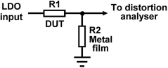
My own measurement setup is shown in Figure 15.5. The resistors are usually of equal value, to give 6 dB attenuation. A very low-distortion oscillator that can give a large output voltage is necessary; the results in Figure 15.6 were taken at a 10 Vrms (+22 dBu) input level. Here thick-film SM and through-hole resistors are compared. The gen-mon trace at the bottom is the record of the analyser reading the oscillator output and is the measurement floor of the AP System I used. The THD plot is higher than this floor, but this is not due to distortion. It simply reflects the extra Johnson noise generated by two 10 kΩ resistors. Their parallel combination is 5 kΩ, and so this noise is at −115.2 dBu. The SM plot, however, is higher again, and the difference is the distortion generated by the thick-film component.

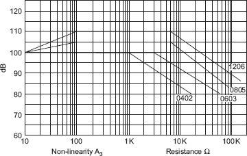
For both thin-film and thick-film SM resistors non-linearity increases with resistor value and also increases as the physical size (and hence power rating) of the resistor shrinks. The thin-film versions are much more linear; compare Figures 15.7 and 15.8.

Sometimes it is appropriate to reduce the non-linearity by using multiple resistors in series. If one resistor is replaced by two with the same voltage coefficient in series, the THD in the current flowing is halved. Similarly, using three resistors reduces THD to a third of the original value. There are obvious economic limits to this sort of thing, and it takes up PCB area, but it can be useful in specific cases, especially where the voltage rating of the resistor is a limitation.

Capacitors: Values and Tolerances

The need for specific capacitor ratios creates problems, as capacitors are available in a much more limited range of values than resistors, usually the E6 series, running 10, 15, 22, 33, 47, 68. If other values are needed, then they often have to be made up of two capacitors in parallel; this puts up the cost and uses significantly more PCB area, so it should be avoided if possible, but for applications like Sallen & Key lowpass filters where a capacitance ratio of 2 is required, it is often the only way. Sallen & Key filters with equal component values can be used (see Chapters 8 and 9), but they must be configured to give voltage gain, which is often unwanted and will force compromises over either noise performance or headroom. Selecting convenient capacitor values will almost invariably lead to a need for non-standard resistance values, but this is much less of a problem, as combining two resistors to get the right value is much cheaper and uses less PCB area.

As for the case of resistors, when contriving a particular capacitor value, the best resolution is obtained by using one large value and one small one to make up the total, but two capacitors of approximately the same value give better average accuracy. When the two capacitors used are equal in nominal value, the accuracy is improved by √2. This effect is more important for capacitors because the cost premium for 1% parts is considerable, whereas for resistors it is very small, if it exists at all. When using multiple components like this to make up a value or improve precision, it is important to keep an eye on both the extra cost and the extra PCB area occupied.

The tolerance of non-electrolytic capacitors is usually in the range ±1% to ±10%; anything more accurate than this tends to be very expensive. Electrolytic capacitors used to have much wider tolerances, but things have recently improved, and ±20% is now common. This is still wider than any other component you are likely to use in a crossover, but this is not a problem, for as described later, it is most unwise to try to define frequencies or time-constants with electrolytic capacitors.

Obtaining Arbitrary Capacitance Values

The problem of making up an arbitrary capacitance value is very different from making up a resistance values. Two things are different:

1. Capacitors are often only available in the E3 or E6 series. Sometimes you can get E12, but rarely E24.
2. Capacitors are significantly more expensive, so using them in multiples is less favourable economically.

There are often different options for capacitor values when designing active crossover filters. For example, you might start your calculations with 1 kΩ resistors, and you find that the biggest capacitor comes out at, say, 450 nF. That can be changed to give the same response using the E3 preferred value of 470 nF by scaling the resistors; here 1 kΩ scaled by 450/470 is 957 Ω. The 2xE24 parallel combination of 1600 Ω and 2400 Ω is only 0.31% high in nominal value. Since the resistor value is slightly reduced, you need to check that the loading on the previous stage has not become excessive.

Alternatively, you might decide to make up the capacitance with two 220 nF capacitors in parallel, to give an improvement in effective tolerance of √2. Now 440 nF is less than 450 nF, so to get the same response the resistors must be scaled up by 450/440, which works out as 1.022 kΩ. The 2xE24 parallel combination of 1300 Ω and 4700 Ω is only 0.36% low in nominal value.

Decisions like this can only be made intelligently if you know the cost of the various options. Resistors cost the same whatever their value, so that simplifies matters. The cost of a capacitor, however, is a strong function of its value. I have tried to give a handle on this in Table 15.15, which gives the relative cost of capacitors at 63 V DC rating and 2% tolerance. Prices were obtained for production quantities as close as possible to 1000-off. These figures are distinctly approximate, as it proved difficult to cross-reference various manufacturers, price breaks, and so on. Some things are, however, clear; for polyester, cost increases more slowly than proportionally with capacitance, very roughly in a square root law. Polypropylene cost increases faster with capacitance but still significantly more slowly than proportionally. Therefore, making up a capacitance with two equal values, as in our example of 440 nF = 2 × 220 nF, is going to cost more than using a single 470 nF capacitor. The table also demonstrates that polypropylene capacitors cost a lot more than polyester, so the cost difference is much greater. In making your design decisions you will of course be working with prices from your intended supplier.

Polypropylene capacitors are much more expensive than polyester, but their great advantage is that they do not generate distortion (see later). In many filter types only one of the capacitors needs to be polypropylene for capacitor distortion to be eliminated, and this can save some serious money. This intriguing state of affairs is described in detail in Chapter 11.

Capacitor Shortcomings

Capacitors fall short of being an ideal circuit element in several ways, notably leakage, equivalent series resistance (ESR), equivalent series inductance (ESL), dielectric absorption, and non-linearity: Capacitor leakage is equivalent to a high value resistance across the capacitor terminals, which allows a trickle of current to flow when a DC voltage is applied. Leakage is usually negligible for non-electrolytics, but is much greater for electrolytics. It is not normally a problem in audio design.

Equivalent series resistance (ESR) is a measure of how much the component deviates from a mathematically pure capacitance. The series resistance is partly due to the physical resistance of leads and foils and partly due to losses in the dielectric. It can also be expressed as tan-δ (tan-delta), which is the tangent of the phase angle between the voltage across and the current flowing through the capacitor. Once again it is rarely a problem in the audio field, the values being small fractions of an ohm and very low compared with normal circuit resistances.

Equivalent series inductance (ESL) is always present. Even a straight piece of wire has inductance, and any capacitor has lead-out wires and internal connections. The values are normally measured in nanohenries and have no effect in normal audio circuitry.

Dielectric absorption is a well-known effect; take a large electrolytic, charge it up, and then fully discharge it. Over a few minutes the charge will partially reappear. This “memory effect” also occurs in non-electrolytics to a lesser degree; it is a property of the dielectric and is minimised by using polystyrene, polypropylene, NP0 ceramic, or PTFE dielectrics. Dielectric absorption is invariably modelled by adding extra resistors and capacitances to an ideal main capacitor, such as Figure 15.9 for a 1 uF polystyrene capacitor, which does not hint at any source of non-linearity. [12] However, the dielectric absorption mechanism does seem to have some connection with capacitor distortion, since the dielectrics that show the least dielectric absorption also show the lowest non-linearity. Dielectric absorption is a major consideration in sample-and-hold circuits but of no account in itself for normal linear audio circuitry; you can see from Figure 15.9 that the additional components are relatively small capacitors with very large resistances in series, and the effect these could have on the response of a filter is microscopic, and far smaller than the effects of component tolerances. Note that the model is just an approximation and is not meant to imply that each extra component directly represents some part of a physical process.

Capacitor non-linearity is the least known but by far the most troublesome of capacitor shortcomings. An RC lowpass filter to demonstrate the effect can be made with a series resistor and a shunt polyester capacitor, as in Figure 15.10, and if you examine the output with a distortion analyser, you will find to your consternation that the circuit is not linear. If the capacitor is a non-electrolytic type with a dielectric such as polyester, then the distortion is relatively pure third harmonic, showing that the effect is symmetrical. For a 10 Vrms input, the THD level may be 0.001% or more. This may not sound like much, but it is substantially greater than the midband distortion of a good opamp. The definitive work on capacitor distortion is a magnificent series of articles by Cyril Bateman in Electronics World. [13] The authority of this is underpinned by Cyril’s background in capacitor manufacture.

Capacitors are used in audio circuitry for four main functions, where their possible non-linearity has varying consequences:

1. Coupling or DC-blocking capacitors. These are usually electrolytics, and if properly sized have a negligible signal voltage across them at the lowest frequencies of interest. The non-linear properties of the capacitor are then unimportant unless current levels are high; power amplifier output capacitors can generate considerable midband distortion. [14] This makes you wonder what sort of non-linearity is happening in those big non-polarised electrolytics in passive crossovers. A great deal of futile nonsense has been talked about the mysterious properties of coupling capacitors, but it is all total twaddle. How could a component with negligible voltage across it put its imprint on a signal passing through it? For small-signal use, as long as the signal voltage across the coupling capacitor is kept low, non-linearity is not detectable by the best THD methods. The capacitance value is non-critical, as it has to be, given the wide tolerances of electrolytics.

2. Supply filtering or decoupling capacitors. Electrolytics are used for filtering out supply rail ripple, etc, and non-electrolytics, usually around 100 nF, are used to keep the supply impedance low at high frequencies and thus keep opamps stable. The capacitance value is again non-critical.

3. For active crossover purposes, by far the most important aspect of capacitors is their role in active filtering. This is a much more demanding application than coupling or decoupling, for first, the capacitor value is now crucially important, as it defines the accuracy of the frequency response. Second, there is by definition a significant signal voltage across the capacitor, and so its non-linearity can be a serious problem. Non-electrolytics are always used in active filters, though sometimes a time-constant involving an electrolytic is ill-advisedly used to define the lower end of the system bandwidth; this is a very bad practice, because it is certain to introduce significant distortion at the bottom of the frequency range.

4. Small value ceramic capacitors are used for opamp compensation purposes, and sometimes in active filters in the HF path of a crossover. So long as they are NP0 (C0G) ceramic types, their non-linearity should be negligible. Other kinds of ceramic capacitor, using the XR7 dielectric, will introduce copious distortion and must never be used in audio paths. They are intended for high-frequency decoupling, where their linearity or otherwise is irrelevant.

Non-Electrolytic Capacitor Non-Linearity

It has often been assumed that non-electrolytic capacitors, which generally approach an ideal component more closely than electrolytics and have dielectrics constructed in a totally different way, are free from distortion. It is not so. Some non-electrolytics show distortion at levels that is easily measured and can exceed the distortion from the opamps in the circuit. Non-electrolytic capacitor distortion is essentially third harmonic, because the non-polarised dielectric technology is basically symmetrical. The problem is serious, because non-electrolytic capacitors are commonly used to define time-constants and frequency responses (in RIAA equalisation networks, for example) rather than simply for DC blocking.

Very small capacitances present no great problem. Simply make sure you are using the C0G (NP0) type, and so long as you choose a reputable supplier, there will be no distortion. I say “reputable supplier” because I did once encounter some allegedly C0G capacitors from China that showed significant non-linearity. [15]

Middle-range capacitors, from 1 nF to 1 uF, present more of a problem. Capacitors with a variety of dielectrics are available, including polyester, polystyrene, polypropylene, polycarbonate, and polyphenylene sulphide, of which the first three are the most common (note that what is commonly called “polyester” is actually polyethylene terephthalate, PET).

Figure 15.10 shows a simple lowpass filter circuit which, with a good THD analyser, can be used to measure capacitor distortion. The values shown give a measured pole frequency, or −3 dB roll-off point, at 723 Hz. We will start off with polyester, the smallest, most economical, and therefore the most common type for capacitors of this size.

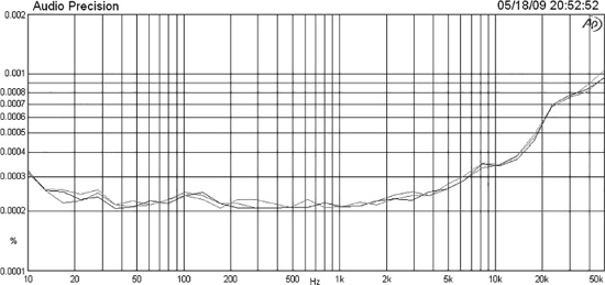
The THD results for a microbox 220 nF 100 V capacitor with a polyester dielectric are shown in Figure 15.11, for input voltages of 10, 15 and 20 Vrms. They are unsettling.

The distortion is all third-harmonic. It peaks at around 300 to 400 Hz, well below the −3 dB frequency, and even with the input limited to 10 Vrms will exceed the non-linearity introduced by opamps such as the 5532 and the LM4562. Interestingly, the peak frequency changes with applied level. Below the peak, the voltage across the capacitor is roughly constant, but distortion falls as frequency is reduced, because the increasing impedance of the capacitor means it has less effect on a circuit node at a 1 kΩ impedance. Above the peak, distortion falls with increasing frequency because the lowpass circuit action causes the voltage across the capacitor to fall.

The level of distortion varies with different samples of the same type of capacitor; six of the type in Figure 15.11 were measured, and the THD at 10 Vrms and 400 Hz varied from 0.00128% to 0.00206%. This puts paid to any plans for reducing the distortion by some sort of cancellation method.

The distortion can be seen in Figure 15.11 to be a strong function of level, roughly tripling as the input level doubles. Third-harmonic distortion normally quadruples for doubled level, so there may well be an unanswered question here. It is however clear that reducing the voltage across the capacitor reduces the distortion. This suggests that if cost is not the primary consideration, it might be useful to put two capacitors in series to halve the voltage and the capacitance, and then double up this series combination to restore the original capacitance, giving the series-parallel arrangement in Figure 15.12. The results are shown in Table 15.16, and once more it can be seen that halving the level has reduced distortion by a factor of three rather than four.

The series-parallel arrangement has obvious limitations in terms of cost and PCB area occupied but might be useful in some cases. It has the advantage that, as described earlier in the chapter, using multiple components improves the average accuracy of the total value.

An unexpected complication in these tests was that every time a polyester sample was remeasured, the distortion was lower than before. I found a steady reduction in distortion over time; if a test signal was applied continuously, 9 Vrms at 1 kHz would roughly halve the THD over 11 hours. This change consists of both temporary and permanent components. When the signal is removed, over days the distortion increases again but never rises to its original value. When the signal is reapplied, the distortion slowly falls again. This self-improvement effect is therefore of little practical use, but if nothing else it demonstrates that polyester capacitors are more complicated than you might think. I do not believe this has anything to do with dim-witted audio commentators claiming that circuitry has to be left switched on for months or years before it attains its optimum sound; for one thing, nothing happens unless you also continuously apply a signal of much higher amplitude than normal, which would be hard to arrange and has never been touted as a good way to run-in equipment. For fuller details of this strange self-improvement business, see my Linear Audio article. [16]

Clearly polyester capacitors can generate significant distortion, despite their extensive use in audio circuitry of all kinds. The next dielectric we will try is polystyrene. Capacitors with a polystyrene dielectric are extremely useful for some filtering and RIAA equalisation applications because they can be obtained at a 1% tolerance at up to 10 nF at a reasonable price. They can be obtained in larger sizes but at much higher prices.

The distortion test results are shown in Figure 15.13 for three samples of a 4n7 2.5% capacitor; the series resistor R1 has been increased to 4.7 kΩ to keep the −3 dB point inside the audio band, and it is now at 7200 Hz. Note that the THD scale has been extended down to a subterranean 0.0001%, because if it was plotted on the same scale as Figure 15.11 it would be bumping along the bottom of the graph. Figure 15.13 in fact shows no distortion at all, just the measurement noise floor, and the apparent rise at the HF end is simply due to the fact that the output level is decreasing because of the lowpass action, and so the noise floor is relatively increasing. This is at an input level of 10 Vrms, which is about as high as might be expected to occur in normal opamp circuitry. The test was repeated at 20 Vrms, which might be encountered in discrete circuitry, and the results were the same, yielding no measurable distortion.

The tests were done with four samples of 10 nF 1% polystyrene from LCR at 10 Vrms and 20 Vrms, with the same results for each sample. This shows that polystyrene capacitors can be used with confidence; this finding is in complete agreement with Cyril Bateman’s results. [17]

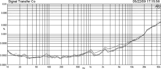
Having resolved the problem of capacitor distortion below 10 nF, we need now to tackle it for larger capacitor values. Polyester having proven unsatisfactory, the next most common capacitor type is polypropylene, and I am glad to report that these are effectively distortion free in values up to 220 nF. Figure 15.14 shows the results for four samples of a 220 nF 250 V 5% polypropylene capacitor from RIFA. The plot shows no distortion at all, just the noise floor, with the apparent rise at the HF end being increasing relative noise due to the lowpass roll-off, as in Figure 15.13. This is also in agreement with Cyril Bateman’s findings. [18] Rerunning the tests at 20 Vrms gave the same result—no distortion. This is very pleasing, but there is a downside. Polypropylene capacitors of this value and voltage rating are much larger physically than the commonly used 63 or 100 V polyester capacitor, and more expensive.

It was therefore important to find out if the good distortion performance was a result of the 250 V rating, and so I tested a series of polypropylene capacitors with lower voltage ratings from different manufacturers. Axial 47 nF 160 V 5% polypropylene capacitors from Vishay proved to be THD-free at both 10 Vrms and 20 Vrms. Likewise, microbox polypropylene capacitors from 10 nF to 47 nF with ratings of 63 V and 160 V from Vishay and Wima proved to generate no measurable distortion, so the voltage rating appears not to be an issue. This finding is particularly important, because the Vishay range has a 1% tolerance, making them very suitable for precision filters and equalisation networks. The 1% tolerance is naturally reflected in the price.

The higher values of polypropylene capacitors (above 100 nF) appear to be currently only available with 250 V or 400 V ratings, and that means a physically big component. For example, the EPCOS 330 nF 400 V 5% part has a footprint of 26 mm by 6.5 mm, with a height of 15 mm, and capacitors like that take up a lot of PCB area. One way of dealing with this is to use a smaller capacitor in a capacitance multiplication configuration, so a 100 nF 1% component could be made to emulate 330 nF. It has to be said that this is only straightforward if one end of the capacitor is connected to ground; see Chapter 14 for an example of this concept applied to a biquad equaliser.

When I first started looking at capacitor distortion, I thought that the distortion would probably be lowest for the capacitors with the highest voltage rating. I therefore tested some RF-suppression X2 capacitors, rated at 275 Vrms, equivalent to a peak or DC rating of 389 V. The dielectric material is unknown. An immediate snag is that the tolerance is 10 or 20%, not exactly ideal for precision filtering or equalisation. A more serious problem, however, is that they are far from distortion free. Four samples of a 470 nF X2 capacitor showed THD between 0.002% and 0.003% at 10 Vrms. A high-voltage rating alone does not mean low distortion.

For more information on how capacitor non-linearity affects filters see Chapter 11.

Electrolytic Capacitor Non-Linearity

Cyril Bateman’s series in Electronics World [17][18] included two articles on electrolytic capacitor distortion. It proved to be a complex subject, and many long-held assumptions, such as “DC biasing always reduces distortion”, were shown to be quite wrong (my own results confirm this—DC biasing is at best pointless and can increase distortion). The distortion levels Cyril measured were in general a good deal higher than for non-electrolytic capacitors, and I can confirm that too.

My view is that electrolytics should never, ever, under any circumstances, be used to set important time-constants in audio. There should be a dominant time-constant early in the signal path, based on a non-electrolytic capacitor, that determines the lower limit of the system bandwidth; preferably proper bandwidth definition should be implemented with a subsonic filter. All the electrolytic-based time-constants should be much longer so that the electrolytic capacitors can never have significant signal voltages across them and so never generate detectable distortion. Electrolytics have large tolerances and cannot be used to set accurate time-constants anyway.

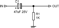
However, even if you think you are following this plan, you can still get into trouble. Figure 15.15 shows a simple highpass test circuit representing an electrolytic capacitor in use for coupling or DC blocking. The load of 1 kΩ is the sort of value that can easily be encountered if you are using low-impedance design principles. The calculated −3 dB roll-off point is 3.38 Hz, so the attenuation at 10 Hz, at the very bottom of the audio band, will be only 0.47 dB; at 20 Hz it will be only 0.12 dB, which is surely a negligible loss. As far as frequency response goes, we are doing fine. But … examine Figure 15.16, which shows the measured distortion of this arrangement. Even if we limit ourselves to a 10 Vrms level, the distortion at 50 Hz is 0.001%, already above that of a good opamp. At 20 Hz it has risen to 0.01%, and at 10 Hz is a most unwelcome 0.05%. The THD is increasing by a ratio of 4.8 times for each octave fall in frequency, in other words increasing faster than a square law. The distortion residual is visually a mixture of second and third harmonic, and the levels proved surprisingly consistent for a large number of 47 uF 25 V capacitors of different ages and from different manufacturers.

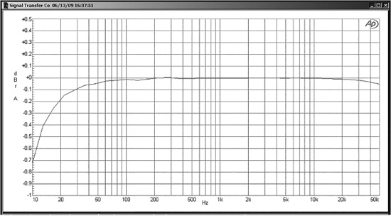
Figure 15.16 also shows that the distortion rises rapidly with level; at 50 Hz, going from an input of 10 Vrms to 15 Vrms almost doubles the THD reading. To underline the point, consider Figure 15.17, which shows the measured frequency response of the circuit with 47 uF and 1 kΩ; note the effect of the capacitor tolerance on the real versus calculated response. The roll-off that does the damage, by allowing an AC voltage to exist across the capacitor, is very modest indeed, less than 0.2 dB at 20 Hz.

Having demonstrated how insidious this problem is, how do we fix it? As we have seen, changing capacitor manufacturer is no help. Using 47 uF capacitors of higher voltage also does not work—tests showed there is very little difference in the amount of distortion generated. An exception was the sub-miniature style of electrolytic, which was markedly more non-linear than standard types.

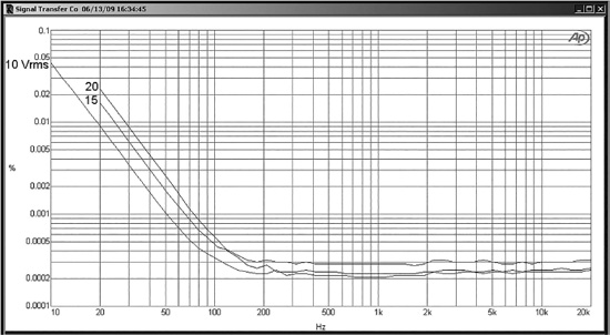
The answer is simple—just make the capacitor bigger in value. This reduces the voltage across it in the audio band, and since we have shown that the distortion is a strong function of the voltage across the capacitor, the amount produced drops more than proportionally. The result is seen in Figure 15.18, for increasing capacitor values with a 10 Vrms input.

Replacing C1 with a 100 uF 25 V capacitor drops the distortion at 20 Hz from 0.0080% to 0.0017%, an improvement of 4.7 times; the voltage across the capacitor at 20 Hz has been reduced from 1.66 Vrms to 790 mVrms. A 220 uF 25 V capacitor reduces the voltage across itself to 360 mV and gives another very welcome reduction to 0.0005% at 20 Hz, but it is necessary to go to 1000 uF 25 V to obtain the bottom trace, which is the only one indistinguishable from the noise floor of the AP-2702 test system. The voltage across the capacitor at 20 Hz is now only 80 mV. From this data, it appears that the AC voltage across an electrolytic capacitor should be limited to below 80 mVrms if you want to avoid distortion. I would emphasise that these are ordinary 85°C rated electrolytic capacitors, and in no sense special or premium types.

This technique can be seen to be highly effective, but it naturally calls for larger and somewhat more expensive capacitors and larger footprints on a PCB. This can be to some extent countered by using capacitors of lower voltage, which helps to bring back down the CV product and hence the can size. I tested 1000 uF 16 V and 1000 uF 6V3 capacitors, and both types gave exactly the same results as the 1000 uF 25 V part in Figure 15.18, which seems to indicate that the maximum allowable signal voltage across the capacitor is an absolute value and not relative to the voltage rating. Naturally, 1000 uF 16 V and 1000 uF 6 V3 capacitors gave very useful reductions in CV product, can size, and PCB area occupied. This does of course assume that the capacitor is, as is usual, being used to block small voltages from opamp offsets to prevent switch clicks and pot noises rather than for stopping a substantial DC voltage.

The use of large coupling capacitors in this way does require a little care, because we are introducing a long time-constant into the circuit. Most opamp circuitry is pretty much free of big DC voltages, but if there are any, the settling time after switch-on may become undesirably long.

References

[1]Smith, Warren J. “Modern Optical Engineering” McGraw-Hill, 1990, ISBN: 0-07-059174-1, p. 484
[2]Johnson, Howard www.edn.com/article/509250-7_solution.php, June 2010
[3]Kroeze, Hugowww.rfglobalnet.com/forums/Default.aspx?gposts&m61096(inactive) March 2002
[4]www.voidware.com/calcs/fx19.htm; Accessed January 2017
[5]Lovell, Mark and Jones, Morgan www.pmillett.com/rescalc.htm
[6]Self, Douglas www.douglas-self.com/
[7]Self, Douglas “Small Signal Audio Design” Second Edn, Focal Press, 2015, Chapter 8, pp. 265–268, ISBN 978-0-415-70974-3 hardback
[8]The Signal Transfer Company www.signaltransfer.freeuk.com/
[9]Self, Douglas “Small Signal Audio Design Handbook” Second Edn, Focal Press, 2015, pp. 321–324, ISBN: 978-0-415-70974-3 hbk
[10]https://en.wikipedia.org/wiki/Th%C3%A9venin’s_theorem; Accessed January 2017
[11]Self, Douglas “Audio Power Amplifier Design” Sixth Edn, Newnes, 2013, pp. 39–45, ISBN: 978-0-240-52613-3
[12]Kundert, Ken “Modelling Dielectric Absorption in Capacitors” www.designers-guide.org/Modeling/da.pdf, 2008
[13]Bateman, Cyril “Capacitor Sound?” Parts 1–6, Electronics World, July 2002–March 2003
[14]Self, Douglas “Audio Power Amplifier Design” Sixth Edn, Newnes, 2013, pp. 107–108, (amp output cap), ISBN: 978-0-240-52613-3
[15]Self, Douglas “Audio Power Amplifier Design” Sixth Edn, Newnes, 2013, pp. 299–300 (C0G cap), ISBN: 978-0-240-52613-3
[16]Self, Douglas “Self-Improvement for Capacitors” Linear Audio, Volume 1, April 2011, p156 ISBN 9–789490–929022
[17]Bateman, Cyril “Capacitor Sound?” Part 3. Electronics World, October 2002, pp. 16, 18
[18]Bateman, Cyril “Capacitor Sound?” Part 4, Electronics World, November 2002, p. 47