Chapter 12

Bandpass and Notch Filters

This chapter deals with bandpass and notch filters. Bandpass filters as such are rarely used in performing the basic band-splitting functions of a crossover, but they can be useful for equalisation purposes and are essential for putting together high-order allpass filters for time correction. Bandpass filters are essential for filler-driver crossover schemes. Notch filters can also be useful for equalisation, but their most important use is in the construction of notch crossovers, whether based on elliptical filters or other sorts of filtering.

Multiple-Feedback Bandpass Filters

When a bandpass filter of modest Q is required, the multiple-feedback or Rauch type shown in Figure 12.1 has many advantages. The capacitors are equal and so can be made any preferred value. The opamp is working with shunt feedback and so has no common-mode voltage on the inputs, which avoids one source of distortion. It does however phase-invert, which can be inconvenient. Phase inversions are no problem in passive crossovers—you simply swap over the wires to the speaker unit—but in an active crossover an extra inverting stage may be needed to undo the first inversion.

Figure 12.1 shows the normal configuration of an MFB or Rauch filter. The minimum Q that can be normally achieved is 0.707 (1/√2), which requires R2 to be set to infinity, i.e. not fitted at all. If you want a lower Q than that, you still omit R2, but the vital point is that a different set of design equations are used that give different values for the other components and allow lower Q’s to be realised. These lower Q’s are required for time-delay compensation allpass filters and for filler-driver crossovers. The design process is fully described in Chapter 13 on time-domain filtering, where low Q’s are especially necessary. This no-R2 variation on the standard MFB filter is sometimes called a Deliyannis filter.

Note that the Deliyannis filter is not suitable for high Q’s, because as the Q is increased, the passband gain increases with it; it cannot be controlled independently, as it can in the standard MFB filter. This will lead to either headroom problems or, alternatively, noise problems if the signal is attenuated before it reaches the filter.

The filter response is defined by three parameters—the centre frequency f₀, the Q, and the passband gain (i.e. the gain at the response peak) A. The filter in Figure 12.1 was designed for f₀ = 250 Hz, Q = 2, and A = 1 using the design equations shown, and the usual awkward resistor values emerged. The resistors shown in Figure 12.1 are the nearest E96 values, and the simulated results come out as f₀ = 251 Hz, Q = 1.99, and A = 1.0024, which, as they say, is good enough for rock ’n’ roll. Using 2xE24 parallel pairs would give even more accurate values.

The Q of the filter can be quickly checked from the response curve, as Q is equal to the centre frequency divided by the −3 dB bandwidth, i.e. the frequency difference between the two −3 dB points on either side of the peak. This configuration is not suitable for Qs greater than about 10, as the filter characteristics become unduly sensitive to component tolerances. If independent control of f₀ and Q are required, the state-variable filter should be used instead.

Figure 12.1: An MFB or Rauch bandpass multiple-feedback filter with f₀ = 250 Hz, Q = 2 and a gain of 1.

Similar MFB configurations can be used for lowpass and highpass filters; see Chapter 10. The lowpass MFB filter does not depend on a low opamp output impedance to maintain stopband attenuation at high frequencies and so avoids the oh-no-it’s-coming-back-up-again behaviour of Sallen & Key lowpass filters. The highpass MFB filter has some unresolved issues with noise and distortion.

High-Q Bandpass Filters

As we have just seen, the simple MFB/Rauch filter is not suitable for high Q’s. When these are required (which is not likely to be very often in crossover design), there are many, many kinds of active filter that can be used. We will just take a quick look at one of the most useful, the double-amplifier bandpass or DABP filter; this is a good example of the way that active filter performance can sometimes be transformed by adding one more inexpensive opamp section. Figure 12.2 shows the circuit with values for a centre frequency of 1 kHz and an impressively high Q of 70, A2 being used to provide one of the feedback paths. The high value of R1 with respect to the rest of the circuit derives from the high Q.

The design equations are pleasantly straightforward; just choose a preferred value for C1 = C2 = C, calculate the value of R and then derive the values of R1, R2, R3 from it. R4 and R5 are non-critical so long as they are of equal value; as usual they should be made as low as possible without overloading A1 output, in order to keep down both their Johnson noise and the effect of the current noise flowing through them from the A2 non-inverting input. In this case R4 and R5 could be reduced to 1 kΩ so long as the external loading on A1 is not too great.

The gain at resonance is always two times (+6 dB), which is very often not wanted. The most convenient way to introduce a compensating 6 dB of attenuation is to split R1 into two resistors which have in parallel the same value as R1, and connect one of them to ground. This technique is also described in Chapter 8 on lowpass filters

Figure 12.3 shows the satisfyingly sharp resonance at a Q of 70 obtained with the circuit of Figure 12.2. Away from the peak, the filter slopes slowly merge into straight lines at 6 dB/octave, as is normal for 2nd-order bandpass responses. Fourth-order bandpass filters with 12 dB/octave skirt slopes can be made by cascading two 2nd-order bandpass filters.

Figure 12.2: Dual-amplifier bandpass (DABP) filter with a centre frequency of 1 kHz and a Q of 70. The gain at resonance is always +6 dB.

Figure 12.3: Dual-amplifier bandpass (DABP) filter with a centre frequency of 1 kHz and a Q of 70. Gain at resonance peak is +6 Db.

Notch Filters

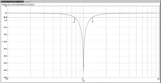
There are a very large number of notch filters, each with their own advantages and disadvantages. The width of a notch is described by its Q. As for a resonance peak, the Q is equal to the centre frequency divided by the −3 dB bandwidth, i.e. the frequency difference between the −3 dB points either side of the notch. Figure 12.4 demonstrates this procedure for a notch with a centre frequency of 1.00 kHz and a Q of 1.5; the bandwidth between the two −3 dB points is 0.667 kHz, so Q = 1.00/0.667 = 1.5. Be aware that the Q of a notch has no special relation to the depth, but if the notch is really shallow—more of a dip than a notch—then the response at the −3 dB points may be affected, and this will affect the calculated Q.

Figure 12.4: Determining the Q of a notch filter, which is equal to the centre frequency divided by the bandwidth between the two −3 dB points.

The symmetrical notch shown in Figure 12.4 is the best-known sort, but there are also highpass notches and lowpass notches. A lowpass notch typically has unity gain on the low-frequency side of the notch and a lower gain on the high-frequency side. A highpass notch typically has unity gain on the high-frequency side of the notch and a lower gain on the low-frequency side. In both cases the responses are flat away from the notch. There is more information on the use of lowpass and highpass notches later in this chapter and in Chapter 5 on notch crossovers.

The Twin-T Notch Filter

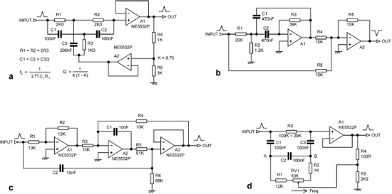
The best-known notch filter is the Twin-T notch network shown in Figure 12.5a, invented in 1934 by Herbert Augustadt. [1] It gives a symmetrical notch. The notch depth is infinite with exactly matched components, but with ordinary ones it is unlikely to be deeper than 40 dB. It requires ratios of two in component values such as 100 Ω–200 Ω, and there are only six such pairs in the E24 resistor series; see Chapter 15. Capacitors have sparser value series, and two will need to be paralleled to get the 1:2 ratio required.

The Twin-T notch when used alone has a Q of only 1/4, which is not very useful. It is therefore normally used with positive feedback via an opamp buffer A2, as shown. The proportion of feedback K and hence the Q-enhancement is set by R4 and R5, which here give a Q of 1. The great drawbacks of the Twin-T are that it depends on matched components for good notch depth and that the notch frequency can only be altered by changing three components, keeping them carefully matched while doing so.

Figure 12.5: Notch filters: (a) Twin-T with positive feedback, notch at 795 Hz and a Q of 1; (b)“1-bandpass” filter with notch at 50 Hz, Q of 2.85; (c) Bainter filter with notch at 700 Hz, Q of 1.29; (d) bridged-differentiator notch filter tuneable 80 to 180 Hz.

The 1-Bandpass Notch Filter

Another way of making notch filters is the “one-minus-bandpass” principle, usually written “1-bandpass” or “1-BP”. The input goes through a bandpass filter, typically the multiple-feedback type described earlier, and is then subtracted from the original signal. The accuracy of the cancellation and hence the notch depth is critically dependent on the midband gain of the bandpass filter. Figure 12.5b shows an example that gives a notch at 50 Hz with a Q of 2.85. The subtraction is performed by A2, as the output of the filter is phase inverted. The multiple-feedback filter is designed for unity passband gain, but the use of E24 values as shown means that the actual gain is 0.97, limiting the notch depth to −32 dB. The value of R6 can be tweaked to deepen the notch; the nearest E96 value is 10.2 kΩ, which gives a depth of −45 dB. The final output is inconveniently phase inverted in the passband.

The Bainter Notch Filter

The Bainter notch filter is a very useful configuration, invented as recently as 1975, [2] making it the newest filter in this book. An example is shown in Figure 12.5c, where the values shown give a symmetrical notch at 700 Hz with a Q of 1.29. You will note that three amplifiers are required, but this is a small price to pay for such a capable filter. The first great advantage is that the depth of the notch does not depend in any way on the matching of components but is determined by the open-loop gain of the amplifiers, being roughly proportional to it; 5532 opamps give a notch depth of about −70 dB with no adjustment at all, while the old TL072 gives less impressive depths of about −40 to −50 dB. Having said that, deep notches are not normally essential for crossover design; even notches that look worryingly shallow usually have a negligible effect on the summed response.

Second, the Bainter notch filter can provide lowpass notches, symmetrical notches, and highpass notches depending on the design decisions (though only one of them at a time). Third, two out of the three amplifiers are working at virtual earth and will give no trouble with common-mode distortion. Fourthly, if it suffers internal clipping this is relatively benign, with only one-sixth of the distortion generated by the clipping amplifier reaching the filter output. Fifthly, the Bainter filter is non-inverting in the passband, which is very handy.

The only real disadvantage of the Bainter filter is that be it set for lowpass, symmetrical, or highpass notch, the gain asymptoted to above the notch frequency is always unity (0 dB), and so making a lowpass notch means having gain on the low-frequency side of the notch, which will often be highly inconvenient in a crossover signal path. About the only other thing I can think of to say against the Bainter is that it is one of those enigmatic configurations which on inspection give very little clue as to how they work. One thing is clear; at frequencies well above the notch, the filter must be unity gain and non-inverting, because then C2 is essentially a short-circuit from the input to the unity-gain buffer, which is connected directly to the output. The signal at the A2 output is then irrelevant, because the resistance of R5 will be much greater than the impedance of C1.

A Bainter filter consists of three opamps, the shunt-feedback stage A1, the integrator A2, and the output buffer A3. See Figure 12.5c. The gain of A1 is here set to unity. You can have any gain here so long as R3 is appropriate to inject the current amount of signal current into the summing point of A2, as noted later, but unity gain is often convenient.

To get a standard symmetrical notch with equal gain either side of the crevasse, R3 must equal R4. R4 greater than R3 gives a lowpass notch, while R3 greater than R4 gives a highpass notch; these responses are useful for making elliptical filters and for other applications in crossover design.

The Bainter filter is usually shown with equal values for C1 and C2. This leads to values for R5 and R6 that are a good deal higher than other circuit resistances, and I suggested in the first edition of this volume that this would impair the noise performance. A bit more thought shows that the junction of R5 and R6 is connected to the input by capacitor C1, and so in the audio band there is no high impedance to generate noise; low-impedance design here will give only a very small noise improvement, if any. The input impedance below the notch is the value of R1. Above the notch it falls to R1 in parallel with R5 and R6, which in most Bainter filters is a very small reduction.

The Bainter filter is set to give a lowpass, symmetrical, or highpass notch by the ratio of the notch frequency f_z to the filter centre frequency f_0. The square of this ratio gives the parameter Z, which is used to calculate R3, R4, and R5 (please note this has nothing whatever to do with using Z to represent impedance). For Z > 1 you get a lowpass notch with R3 < R4. For Z = 1 you get a symmetrical notch with R3 = R4. For Z < 1 you get a highpass notch with R3 > R4. The gain g of the shunt-feedback stage A1 can be set arbitrarily, as it can be allowed for by the value of R3. Unity gain seems to give good results for noise and distortion, but I am not claiming each is always optimal. It occurs to me that suitable adjustment of R3 would allow both R1 and R2 to be preferred values.

The design procedure given here assumes the passband gain is unity. You can get gain by making A3 a series-feedback amplifying stage, but unity gain is usually what’s wanted.

Bainter Notch Filter Design

The design procedure is thus:

1. Choose C = C1 =C2
2. Choose gain of shunt-feedback stage g
   (Different values can be used for C1 and C2, but it makes the calculation more complicated)
3. Choose R1
4. Calculate R2 = gR1
5. Choose the centre frequency of the filter f₀
6. Choose the notch frequency f_Z
   (this is only the notch frequency for a symmetrical notch)
7. Calculate: $Z={\left(\frac{f_z}{f_0}\right)}^2$
8. Calculate α = 2πf₀C
   For Z > 1 you get a lowpass notch
   For Z = 1 you get a symmetrical notch
   For Z < 1 you get a highpass notch
9. Choose Q
   The value of Q that gives maximal flatness in the passband depends on the value of Z
   For Z = 1/2, Q = 1 gives maximal flatness.
10. Calculate $R3=\frac{g}{2ZQa}$ $R4=\frac{1}{2Qa}$ $R5=R6=\frac{2Q}{a}$

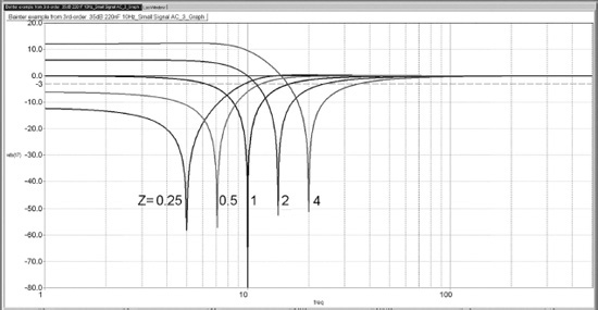
The effect of changing the parameter Z is illustrated in Figure 12.6. For Z > 1 you get a lowpass notch, for Z = 1 you get a symmetrical notch, and for Z < 1 you get a highpass notch, as already noted. The gain is always unity above the notch frequency because of the presence of C2. The symmetrical notch is centred on the low frequency of 10 Hz because these plots were originally part of a subsonic filter development program. The Bainter filter is an extremely convenient building block for highpass filters, but not so much for lowpass filters, because a lowpass notch means gain on the low-frequency side of the notch, and this will often be highly inconvenient.

Figure 12.7 shows the effect of different values of Q with Z = 1/2 to give a highpass notch.

Looking at Figure 12.5c, we can attempt some deductions about the likely distortion performance. I never make predictions, and I never will, but I think we can say:

Figure 12.6: Bainter lowpass, symmetrical, or highpass notches for different values of the parameter Z. Q = 1.

Figure 12.7: Bainter response for different values of Q. Z = 1/2 to give a highpass notch.

1. Opamp A1 is working in shunt-feedback mode, so there is no common-mode (CM) voltage on its inputs, and so no common-mode distortion.
2. A1 is also working at a low noise gain so there will be plenty of negative feedback (NFB) to reduce distortion.
3. A2 is working in shunt-feedback mode, so there is no CM voltage on its inputs.
4. A2 is working as an integrator, so there will be a lot of NFB at high frequencies where open-loop gain is falling.
5. A3 is a voltage-follower, so it has maximal CM voltage on its inputs, which may cause increased distortion.
6. A3 is a voltage-follower, so it has maximal NFB, which should reduce distortion.
7. Perhaps most importantly, in the audio passband the signal only goes through C2 and A3, so distortion from A1 and A2 does not reach the output.

All these statements except (5) look promising. Now some thoughts about the likely noise performance:

1. A1 has low-value resistors around it, set by R2, which loads its output; 1 kΩ was chosen to give good THD results with 5532 opamps.
2. A1 is in shunt-feedback mode, so it is operating at a higher noise gain than its signal gain, increasing noise.
3. A2 is an integrator, and they are quiet because of low gain at high frequencies.
4. A3 is working at unity signal gain and noise gain, so noise output should be low.
5. Again, perhaps most importantly, over the audio band, A3 is directly connected to the input via C2, so only the input voltage noise of A3 will be seen at the output.

Both sets of predictions were very largely confirmed by the measurements made, confirming that the Bainter filter is an excellent configuration.

Bainter Notch Filter Example

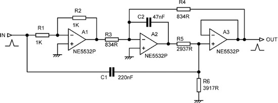
As an example of filter scaling and impedance reduction, a low-noise Bainter filter with a symmetrical notch at 1 kHz and a Q of 2.3 is shown in Figure 12.8. Starting from the circuit of Figure 12.5c with the notch at 700 Hz, both capacitors were scaled by the same ratio to change the notch centre frequency to 1 kHz. The value of R6 was then changed to give the desired Q of 2.3. The first stage of impedance reduction was to reduce R1 and R2 from 10 kΩ to 1 kΩ, which is about as far as you can take it without loading a previous stage excessively. The next stage was to then alter R3, R4 and C2 so that the resistance values were decreased by the same ratio as C2 was increased; this leaves the frequency-dependent behaviour of this network unchanged. The third stage of impedance reduction reduces R6 while increasing C1 by the same ratio, once again keeping the frequency-dependent behaviour the same, though as noted earlier this may not give much lower noise.

The limits of the first impedance reduction are set by the value of R3, which directly loads the output of A1, the value of R4 that loads A3, and the combined value of R5, R6 in series, which loads A2. The last condition is less critical; as you can see from Figure 12.6, the values of R5 and R6 are such as to present only a light load on A2 output, despite the fact that C1 is considerably bigger than C2. A further reduction in R5, R6 would be possible, but C1 then starts to get expensive, and the loading on whatever stage is driving this filter must also be considered.

Figure 12.8: Bainter filter with symmetrical notch at 1 kHz and a Q of 2.3.

An Elliptical Filter Using a Bainter Highpass Notch

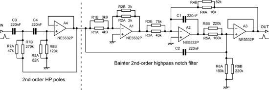
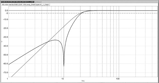
The ability of the Bainter to give either a lowpass or highpass notch makes it a very useful building block for elliptical filters that have a zero or zeros in the stopband. I have made use of this in designing a comprehensive suite of elliptical highpass subsonic filters to assist with vinyl reproduction. [3] What I consider the most effective of these is shown in Figure 12.9, with 2xE24 pairs given for the awkward resistor values. It is a 4th-order elliptical filter with a single stopband notch centred on 10 Hz, where spurious vinyl signals are often at their maximum level due to arm/cartridge resonance. The complete filter consists of a 2nd-order highpass stage A4, placed at the front to reduce internal clipping problems (I call this the New Order) and followed by a Bainter highpass notch. The response is shown in Figure 12.10. The noise output was −113 dBu (22Hz–22kHz, rms sensing) with all opamps 5532. The filter easily handled 10 Vrms in/out at low distortion from 50 Hz to 50 kHz. My recent book Electronics for Vinyl [3] contains much more on subsonic filtering.

I like the Bainter filter. It is a very useful and well-behaved filter configuration. It may not be the simplest of filters, but its inherently deep notch and its good noise and distortion behaviour are a joy to work with. Mr Bainter, I salute you.

There are relatively few references to the Bainter filter in the literature; Valkenburg [4] is one.

The Bridged-Differentiator Notch Filter

A notch filter that can be tuned with one control can be useful in development work. Figure 12.5d shows a bridged-differentiator notch filter tuneable from 80 to 180 Hz by RV1. R3 must theoretically be six times the total resistance between A and B, which here is 138 kΩ, but 139 kΩ gives a deeper notch, about −27 dB across the tuning range. The downside is that Q varies with frequency from 3.9 at 80 Hz to 1.4 at 180 Hz; clearly it is no substitute for a state-variable filter where frequency and Q can be changed independently. It may be an economical circuit in terms of amplifiers, but it uses three capacitors instead of the two in the 1-BP and Bainter filters.

Figure 12.9: Schematic of practical 4th-order A₀ = −35 dB classical highpass elliptical filter, using the New Order.

Figure 12.10: Frequency response of 4th-order A₀ = −35 dB classic (non-MCP) highpass elliptical filter compared with 3rd-order Butterworth. Response is −3 dB at 21 Hz, almost the same as the Butterworth, which is −3 dB at 20 Hz.

Boctor Notch Filters

Another interesting notch filter is the Boctor circuit, which uses only one opamp. [5], [6] Versions exist that can give either a lowpass or highpass notch. The design equations are complicated but can be found in the two references given. Figure 12.11 shows the lowpass and highpass versions.

Figure 12.11: Lowpassnotch (a) and highpass notch (b) Boctor filters. The design at (b) has a notch at 150 Hz with a Q of 1.

Figure 12.12: Response of Boctor filter in Figure 12.7b, giving a highpass notch at 150 Hz with a Q of 1.

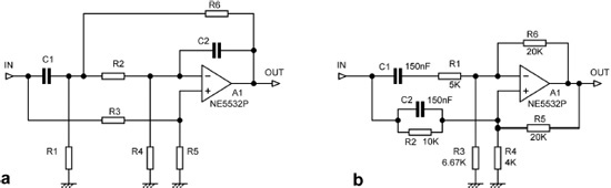
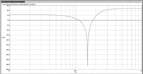
Figure 12.12 shows the highpass notch produced by the Boctor circuit of Figure 12.11b; the high-frequency passband gain is +12 dB, with a gain of +6 dB on the low-frequency side of the notch. The capacitor values may be scaled to change the notch frequency, but they must be the same. A lowpass notch is the mirror image of this sort of response, with the low-gain section on the high-frequency side.

Like Bainter filters, Boctor highpass or lowpass notch filters are frequently used as a component part of elliptical filters.

Other Notch Filters

The field of active filters is rich in possibilities. Other notch filters that there is no space to examine here, but which can be found in the filter textbooks, can be derived from biquad filters such as the Fliege filter, [7] the Tow-Thomas filter, the KHN state-variable filter, the Berka-Herpy filter, the Akerberg-Mossberg filter, and the Natarajan filter; these give symmetrical notches. See Chapter 10 for more on them. Filters apart from the Bainter and the Boctor that can generate highpass or lowpass notches are Friend’s SAB circuit [8] and the Scultety filter. The only reference I can find for the latter is [9], which at least gives the schematic; the same reference also gives schematics of the other filter mentioned in this section.

The Wien-Robinson filter is not biquad-based but uses a Wien network with feedback around it. [10] Notch depth depends on component accuracy, unlike the Bainter, and it seems to have no compensating advantages.

Simulating Notch Filters

When simulating notch filters, assessing the notch depth can be tricky. You need a lot of frequency steps to ensure you really have hit bottom with one of them. For example, in one run, 50 steps/decade showed a −20 dB notch, but upping it to 500 steps/decade revealed it was really −31 dB deep. In most cases having a stupendously deep notch is pointless. If you are trying to remove an unwanted signal, then it only has to alter in frequency by a tiny amount and you are on the side of the notch rather than the bottom, and the attenuation is much reduced. The exception to this is the THD analyser, where a very deep notch (120 dB or more) is needed to reject the fundamental so very low levels of harmonics can be measured. This is achieved by continuously servo-tuning the notch, so it is kept exactly on the incoming frequency.

References

[1]Augustadt, H. Electric Filter US Patent 2,106,785, February 1938, assigned to Bell Telephone Labs
[2]Bainter, J. R. “Active Filter Has Stable Notch, and Response Can Be Regulated” Electronics, pp. 115–117, 2 October 1975
[3]Self, Douglas “Electronics for Vinyl” Taylor & Francis, 2017
[4]Valkenburg, Van “Analog Filter Design”, pp. 346–349
[5]Boctor, S. A. “Single Amplifier Functionally Tuneable Low-Pass Notch Filter” IEEE Trans Circuits & Systems, CAS-22, 1975, pp. 875–881
[6]Valkenburg, Van “Analog Filter Design”, p. 349
[7]Carter and Mancini (ed.) “Opamps for Everyone” Third Edn, Newnes, 2009, Chapter 21, p. 447, ISBN: 978-1-85617-505-0
[8]Valkenburg, Van “Analog Filter Design”, p. 356
[9]www.schematica.com/active_filter_resources/a_list_of_active_filter_circuit_topologies.html; Accessed July 2017
[10]Tietze and Shenk “Electronic Circuits” Second Edn, Springer, 2008, pp. 825–826