6. How We Compute Digital Signal Spectra
Computing Digital Spectra
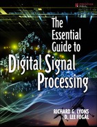
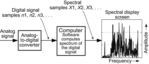
One of the most important aspects of digital signal processing is the computation, and display on a computer screen, of the spectral amplitude of a digital signal as shown in Figure 6-1. The ability to examine the spectrum of a digital signal is as crucial to a signal processing engineer as a microscope is to a medical researcher.
Today, there are two primary methods available to compute digital signal spectra, and those two procedures have the fancy names of the discrete Fourier transform and the fast Fourier transform. This chapter briefly introduces those two functionally equivalent spectral computational methods, and ends with an example of computing a digital signal spectrum for the interested reader.
The Discrete Fourier Transform
The discrete Fourier transform is a mathematical process in which an input sequence of digital signal samples is correlated with an array of digital sine and cosine sequences of different frequencies to compute a new sequence of samples that represents the spectral content of the original digital signal. Whew! That was a mouthful! Let’s just say that the discrete Fourier transform (popularly known as the DFT) is a mathematical process performed on digital signal sequences to compute their spectra, and those spectral results can then be plotted on a computer screen.
Although basically a set of arithmetic comparisons or correlations, the discrete Fourier transform is far too mathematically complicated to describe its inner algebraic details in any meaningful way here. However, we must mention one of the discrete Fourier transform’s important characteristics. Performing a discrete Fourier transform requires an astonishingly large number of arithmetic computations. For example, let’s say we want to compute the spectrum of just a one-second interval of a digital voice signal sampled at a rate of fs = 8,000 Hz. Using the discrete Fourier transform to compute the digital voice signal’s spectrum requires us to perform over 128 million addition operations and over 256 million multiplication operations to compute the spectral X1, X2, X3, . . . sample values as depicted in Figure 6-1. To call this “some serious number crunching” is putting it far too mildly. And the computational workload to obtain the spectrum of longer time-duration signals, sampled at higher fs sample rates, becomes truly astronomical. Fortunately, thanks to the brilliant work of dead mathematicians and the use of modern digital computers, today there is a more efficient way to compute digital signal spectra.
The Fast Fourier Transform
The fast Fourier transform, developed in the United States in the mid-1960s, is an alternate mathematical technique for computing the spectra of digital signals. In fact, the fast Fourier transform (popularly known as the FFT) computes identical results to those computed by the discrete Fourier transform. However, the number of arithmetic computations needed by the fast Fourier transform compared to the discrete Fourier transform is dramatically reduced.
As an example of the fast Fourier transform’s computational efficiency, recall the scenario above where we wanted to compute the spectrum of a one-second interval of a digital voice signal sampled at a rate of fs = 8,000 Hz. Doing this using the fast Fourier transform requires roughly 100,000 addition operations and 200,000 multiplication operations. That’s a computation reduction by a factor of 1,000 compared to the computations required by the discrete Fourier transform. What we’re saying is that for each multiplication operation required by the fast Fourier transform, the discrete Fourier transform requires 1,000 multiplications! Consequently, the fast Fourier transform is the spectral computation method of choice among modern signal processing engineers.
By the Way
The Fourier transform is named after the 19th-century French mathematician and scientist, Jean Baptiste Joseph Fourier. (The name Fourier is pronounced ‘for-YAY, like obey.) A friend of Napoléon Bonaparte, in 1822 Fourier was the first person to propose that periodic waveforms can be described as the sum of various sinusoidal waveforms.
A Spectral Computation Example
This section provides, for those courageous readers willing to continue, a simple example of how the spectrum of a digital signal is computed. In Chapter 3, we discussed a square wave-like analog signal that was the sum of a 2 Hz sine wave plus lower-amplitude 6 Hz and 10 Hz sine waves as shown in Figure 6-2(b). A digital signal version of the composite signal is given in Figure 6-2(c).
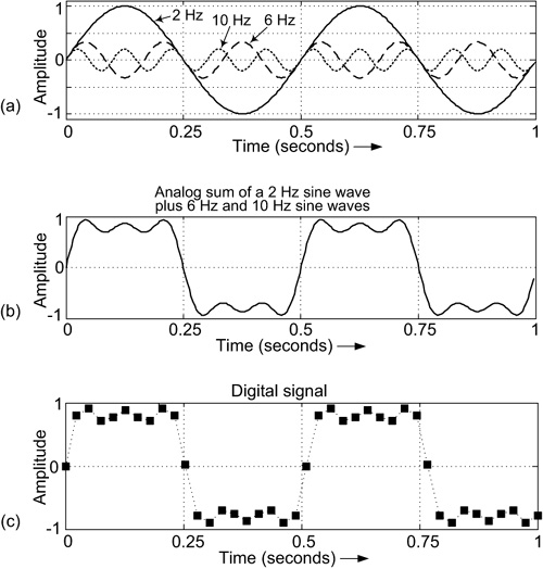
Figure 6-2 A square wave-like signal: (a) individual analog 2 Hz, 6 Hz, and 10 Hz sine waves; (b) analog sum of the sine waves; (c) a digital signal version of the sum of the sine waves sampled at a rate of 40 samples per second (fs = 40 Hz).
The Computations
The goal in our example is to compute the spectrum of the Figure 6-2(c) digital signal. Conceptually, both the discrete Fourier transform and the fast Fourier transform compute the spectrum of the Figure 6-2(c) digital signal sequence as follows:
1. The digital signal sequence has 40 samples; n1, n2, n3, . . . , n40, as shown in Figure 6-3(a). First, we create a single-cycle sine wave sequence having 40 samples as shown in Figure 6-3(b).
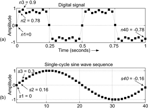
Figure 6-3 Computing the first spectral sample value X1: (a) the digital signal sequence; (b) a single-cycle sine wave sequence.
2. Multiply each sample in the digital signal by its corresponding sample in the single-cycle sine wave sequence, resulting in 40 products. That is, the first product is P1 = n1 × s1. (The “x” means times, a multiplication.) The second product is P2 = n2 × s2, the third product is P3 = n3 × s3, and so on up to the 40th product P40 = n40 × s40.
3. Then, we sum the 40 products to obtain our first spectral sample value X1. That is, X1 = P1 × P2 + P3 + . . . + P40. Because some of the products are positive and some of the products are negative, for our example those products sum to exactly zero. So X1 = 0.
4. Next, create a two-cycle sine wave sequence, having 40 samples, as shown in Figure 6-4(b).
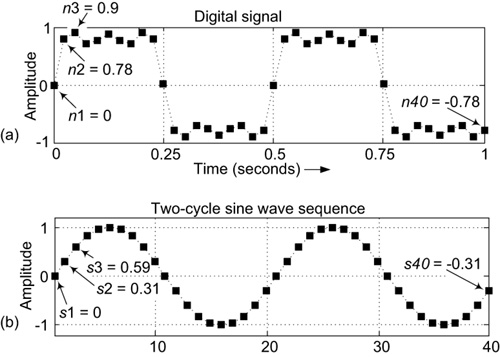
Figure 6-4 Computing the second spectral sample value X2: (a) the digital signal sequence; (b) a two-cycle sine wave sequence.
5. Multiply each sample in the digital signal by its corresponding sample in the two-cycle sine wave sequence, resulting in 40 products. Again, the first product is P1 = n1 × s1. The second product is P2 = n2 × s2, the third product is P3 = n3 × s3, and so on up to the 40th product P40 = n40 × s40.
6. Sum the 40 products to obtain our second spectral sample value. That is, X2 = P1 + P2 + P3 + . . . + P40. For our example, those products sum to 20. So X2 = 20.
7. Next, create a three-cycle sine wave sequence, having 40 samples, as shown in Figure 6-5(b).
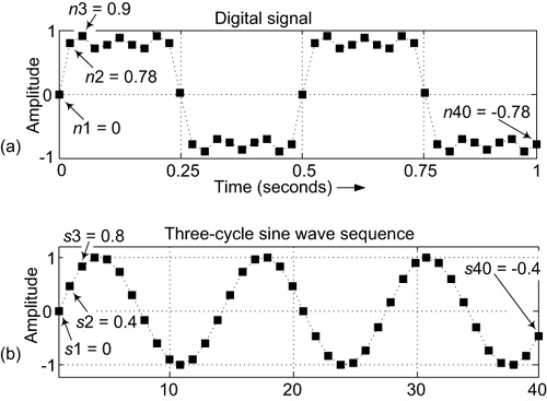
Figure 6-5 Computing the third spectral sample value X3: (a) the digital signal sequence; (b) a three-cycle sine wave sequence.
8. As before, multiply each sample in the digital signal by its corresponding sample in the three-cycle sine wave sequence, again resulting in 40 products.
9. Sum the 40 products to obtain our third spectral sample value X3 = P1 + P2 + P3 + . . . + P40. For our example, those products sum to zero. So X3 = 0.
10. Repeat steps 7 through 9 another 17 times, increasing the number of cycles in the sine wave sequence by one each time, until we have computed 20 spectral samples values, X1 to X20.
11. Plot the 20 spectral samples values on a graph with frequency as the horizontal axis.
Performing the steps above for our square wave-like digital signal gives us the 20 spectral sample values listed in Table 6.1. And, finally, plotting those spectral sample values produces our desired spectral plot shown in Figure 6-6. (Figures 6-6(a) and 6-6(b) show two popular plotting methods. One plot uses dots to represent the spectral samples, and the other plot connects the spectral sample values with solid lines and deletes the dots.) In that figure, we see that the digital signal contained a high-amplitude 2 Hz spectral component, a lower-amplitude 6 Hz spectral component, and a slightly lower-amplitude 10 Hz spectral component. Upon reviewing Figure 6-2(a), we see that our Figure 6-6 spectral results are correct.
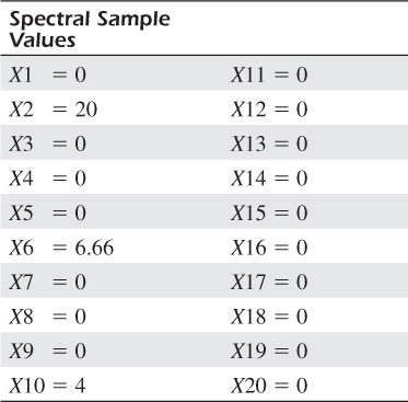
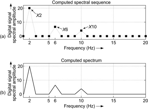
Figure 6-6 Spectrum of the square wave-like digital signal. Two plotting formats: (a) using dots to represent the spectral samples; (b) solid lines connecting the spectral sample values and dots removed.
What the Computations Mean
For the example above, in Figure 6-3 when we multiplied each sample in the digital signal by its corresponding sample in the single-cycle sine wave sequence and summed the 40 products, we arrived at a value of X1 = 0. That summing of products operation gives us a single numerical value, X1 = 0, indicating how well the single-cycle sine wave sequence compared with the square wave-like digital signal. The X1 = 0 value tells us our digital signal compares very poorly with the 1 Hz sine wave sequence. Stated differently, the X1 = 0 value reveals that our digital signal contains a zero amount of 1 Hz spectral energy.
However, in Figure 6-4 we multiplied each sample in the digital signal by its corresponding sample in the two-cycle sine wave sequence and summed the 40 products to yield a value of X2 = 20. The X2 = 20 value tells us our digital signal compares very well with the 2 Hz sine wave sequence. (The peaks and valleys of the two-cycle sine wave sequence are very well aligned with the positive and negative values of our square wave-like digital signal.) That is, the X2 = 20 value reveals that our digital signal contains a large amount of 2 Hz spectral energy.
As we continued our summing of products operations, we found that our numerical comparisons were always zero-valued except when the sine wave sequences had frequencies of 2, 6, and 10 Hz. Therefore, our square wave-like digital signal contained varying amounts of spectral energy at the frequencies of 2, 6, and 10 Hz.
By the Way
Mathematicians have a name for our summation of products operation, and you’ve heard that name before. It’s called correlation. In Chapter 7, Wavelets, we’ll read about comparisons that involve waveforms other than sine waves. Stay tuned.
A Spectral Analysis Example
Let’s consider a real-world spectral analysis example. Think about a large electric motor, shown in Figure 6-7(a), located on the factory floor of a manufacturing company. (By large, we mean, say, the size of a beer keg.) Perhaps the motor drives a heavy-duty hydraulic pump, or maybe a large conveyor belt. In any case, let’s assume the motor’s drive gear turns a larger gear as shown in Figure 6-7(b).
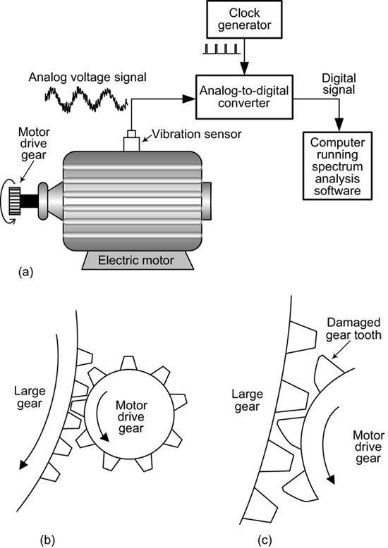
Figure 6-7 Electric motor and gears: (a) motor and vibration test setup; (b) new motor drive gear; (c) worn motor drive gear.
When the motor, and any attached equipment, is first installed, the teeth of the gears mesh very well as shown in Figure 6-7(b). But over time, the drive gear becomes worn as shown in Figure 6-7(c). And when the teeth of the drive gear become badly worn, an unexpected equipment failure can occur—and factory engineers don’t like unexpected equipment failures.
Those clever engineers are able to avoid unexpected electric motor failures by performing spectrum analysis on the vibration of their electric motors. Here’s how: As it turns out, when a new motor, and any connected mechanical equipment, is first installed in a factory, engineers attach a vibration sensor to the motor’s case as shown in Figure 6-7(a). (Just as a microphone converts a sound signal, which consists of fluctuations in air pressure, into a voltage signal, the vibration sensor converts mechanical vibrations into an electrical voltage.) By means of an analog-to-digital converter, the analog vibration signal is converted to a digital signal, which is then passed to a computer. The computer uses fast Fourier transform software to compute and display the vibrational spectrum of a new factory installation. If the motor is rotating at 20 revolutions per second, and the motor’s drive gear has 12 teeth, the vibration spectrum will contain a 20 × 12 × 240 Hz spectral component (in addition to the 20 Hz component from the motor itself) as shown in Figure 6-8(a).
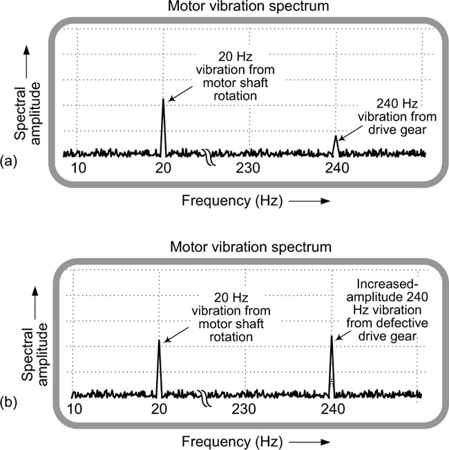
Figure 6-8 Motor vibration spectra: (a) new motor vibration spectrum; (b) worn-gear motor vibration spectrum.
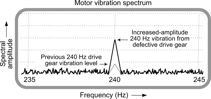
Now when the teeth of the motor’s drive gear become worn, it causes increased motor-case vibration. So some months after installation, the factory engineers repeat their motor vibration spectral test. Let’s say the new spectrum display is that shown in Figure 6-8(b). Seeing an increased amplitude of the 240 Hz spectral component, the engineers zoom in on the spectral display at the 240 Hz frequency as shown in Figure 6-9. From that display, the engineers know that the drive gear’s teeth are becoming worn. This way, the engineers can schedule corrective maintenance that is the least disruptive to the factory’s production process.
What You Should Remember
The concepts you should remember from this chapter are:
• The discrete Fourier transform (DFT) and the fast Fourier transform (FFT) are functionally equivalent mathematical methods for computing the spectra of digital signals.
• The discrete Fourier transform requires a very large number of arithmetic computations.
• The fast Fourier transform requires relatively few arithmetic computations, and is now the most popular method for computing the spectra of digital signals.