8. Digital Filters
In previous chapters, we mentioned the idea of filtering analog and digital signals. Because filtering is a crucial operation in all voice communications, music, and video signal processing systems, let’s learn more about filters and filtering.
The word filter means just what you might expect—a device that allows certain things to pass through and blocks other things. For example, the paper filter in your electric coffee maker allows water to pass through but blocks the coffee grounds. The air filter in your automobile allows air to pass through to your car’s engine but blocks any dust particles.
Instead of water or air, let’s talk about electronic filters that allow certain signal frequencies to pass and block other signal frequencies. In analog signal processing, an analog filter accepts an input analog voltage signal that contains some arbitrary amount of energy at various frequencies and only allows signal energy within a certain frequency range to pass through. In digital signal processing, a digital filter accepts an input digital signal sequence (a list of numbers) that contains some arbitrary amount of energy at various frequencies and only allows signal energy within a certain frequency range to pass through. For example, we may have a voice signal that is contaminated with high-frequency noise. Passing that noisy signal through a filter can eliminate the noise and yield a clean (uncontaminated) voice signal. Let’s clarify this idea of filtering by looking at examples of both analog and digital filters.
Analog Filtering
Analog filters are a collection of interconnected electronic hardware components mounted on a printed circuit board. These filters accept analog voltage signals as inputs and produce altered analog voltage signals as outputs.
As an example of analog filtering, let’s say an engineer wants to build an analog sine wave generator whose frequency is 3 kHz (3,000 Hz). But due to hardware component imperfections, the engineer’s generator output voltage is a badly distorted analog signal as shown in Figure 8-1(a). Looking at the distorted sine wave’s spectrum using an analog spectrum analyzer shows the desired 3 kHz sine wave signal is contaminated with undesired spectral components whose frequencies are 5 kHz and 7 kHz as presented in Figure 8-1(b).
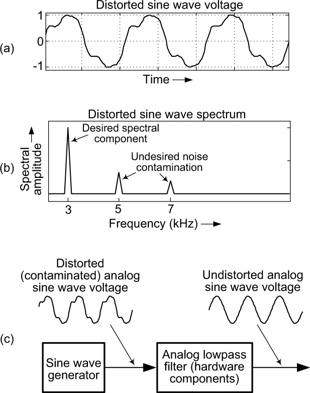
Figure 8-1 A distorted 3 kHz analog sine wave: (a) distorted sine wave voltage; (b) distorted sine wave spectrum; (c) lowpass filtering to produce an undistorted 3 kHz analog sine wave signal.
One solution to the engineer’s sine wave generation problem is to apply the distorted sine wave voltage to an analog lowpass filter that passes the desired 3 kHz spectral energy and blocks the higher-frequency 5 kHz and 7 kHz spectral energy. This scenario is shown in Figure 8-1(c).
If you recall, we’ve already discussed one application of an analog lowpass filter. That was the analog lowpass anti-aliasing filter in Chapter 5’s Figure 5-25(b) digital signal spectrum analysis example.
Generic Filter Types
The filter in Figure 8-1(c) is called a lowpass filter because it passes low frequencies and blocks high frequencies. We show the characteristic of a generic lowpass filter as the frequency-domain curve in Figure 8-2(a). The passband of that curve is the frequency range of signals that will pass through the filter. The stopband of the curve is the frequency range of signals that will be blocked from passing through the filter. For our lowpass filter in Figure 8-1(c), 3 kHz is in the passband of the lowpass filter, and 5 kHz and 7 kHz are in the stopband of the filter.
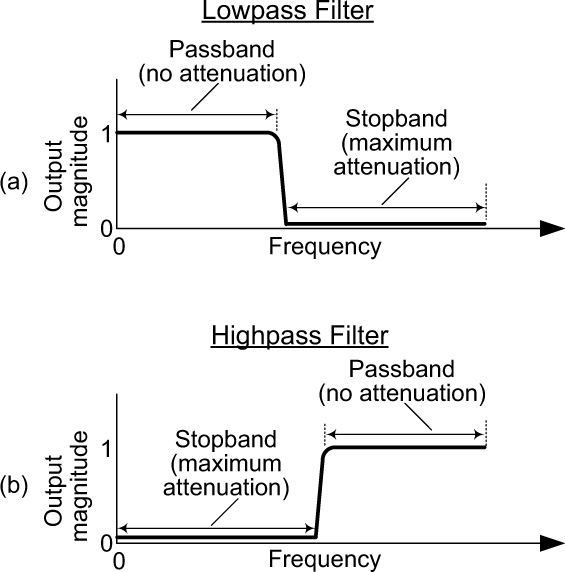
The frequency-domain behavior of a highpass filter is shown in Figure 8-2(b). This figure shows us that a highpass filter allows high-frequency signals to pass through, while it blocks low-frequency signals.
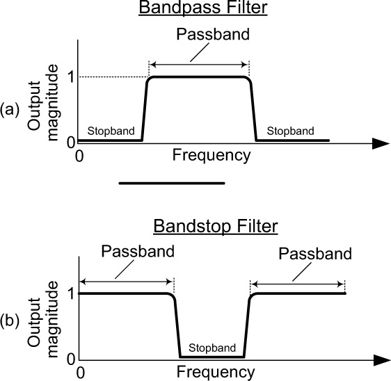
There are two other types of filters used in signal processing: bandpass filters and bandstop filters. The frequency-domain behavior of these filter types is shown in Figure 8-3. Bandpass filters have a passband between two stopbands, while stopband filters have a stopband between two passbands.
It’s important to note that the four generic filter types described above, with their specific passband and stopband locations, can be implemented as either analog or digital filters.
Digital Filtering
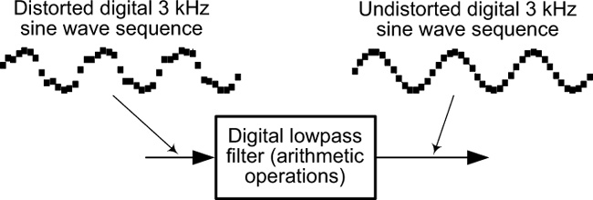
Digital filters share all the behavioral characteristics of analog filters, with two exceptions: first, digital filters operate on digital signals (sequences of numbers); second, digital filters are arithmetic operations rather than electronic hardware components. We illustrate these exceptions by showing a digital signal lowpass filtering process in Figure 8-4, where a noisy digital 3 kHz sine wave signal is filtered to produce a clean sine wave digital signal. That is, arithmetic operations are performed on the input digital signal sequence of numbers to generate a new digital signal sequence of numbers that we treat as the output of the digital filter. Let’s now show the arithmetic details of a simple, real-world digital lowpass filtering example.
Doctors like to obtain their patients’ accurate blood pressure readings. In addition to taking periodic blood pressure readings, your doctor might be looking for any trends such as a slow rise of blood pressure over, say, a year’s time. A single blood pressure reading produces two numbers of interest to a doctor, the systolic and diastolic blood pressure values. However, for this digital filtering example we’ll focus only on the first number, the systolic blood pressure.
Figure 8-5(a) shows a hypothetical sequence of 365 daily systolic blood pressure readings. That sequence is a digital signal and, for clarity, we plot it with straight lines rather than using dots.
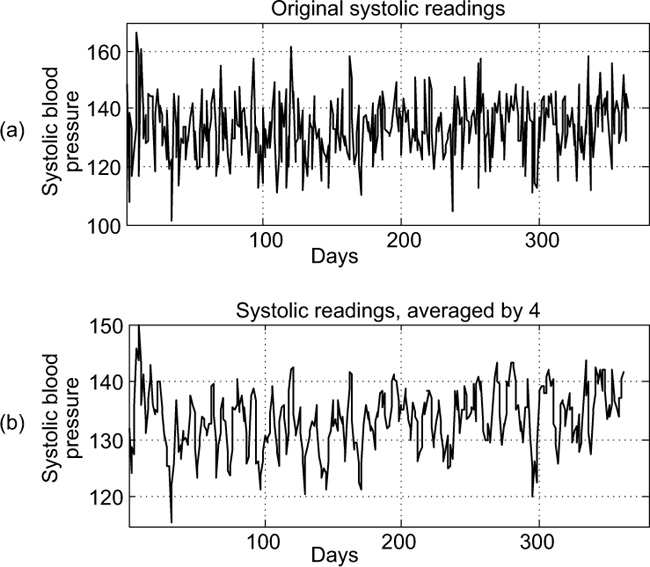
It’s pretty hard to spot any long-term blood pressure trends here because the reading values fluctuate so much, ranging from 101 to 166. The first four readings are 148, 107, 139, and 133. If we average those first four values, we obtain a result of 132. If we average the 2nd, 3rd, 4th, and 5th readings, we obtain a result of 124. When we average the 3rd, 4th, 5th, and 6th readings, we obtain a result of 129. Let’s continue this process of averaging sets of four incremented successive readings for the whole year. This arithmetic process of averaging successive groups of four pressure values is called a moving averager and is one method of lowpass filtering signal data. Figure 8-5(b) shows the results of using this four-point moving averager.
We can see a little smoothing of the averaged values in Figure 8-5(b) where the value fluctuations are reduced. However, a doctor would still be hard pressed to spot any long-term trend in blood pressure readings. If we average a larger number of successive readings, we would achieve better smoothing. Averaging the 1st through the 16th readings, the 2nd through the 17th readings, the 3rd through the 18th readings, and so on produces the sequence of values shown in Figure 8-6(a). There we see further data-value smoothing, in which case a doctor can begin to see an upward trend in blood pressure readings. What we are doing here is lowpass filtering the original blood pressure data sequence to reduce its high frequency value fluctuations.

Going further, we can average our original blood pressure readings in successive sets of 64 contiguous samples. That is, averaging the 1st through the 64th readings, the 2nd through the 65th readings, the 3rd through the 66th readings, and so on. Doing this results in the curve shown in Figure 8-6(b). The reading values are now significantly smoothed and a doctor can easily detect increasing blood pressure over the period of one year. Again, this long-term upward trend was not noticeable in the original blood pressure readings shown in Figure 8-5(a).
At the beginning of this section, we stated that digital filters are essentially arithmetic operations. And the blood pressure numerical averaging operations discussed above are forms of digital lowpass filtering. It’s important to realize that there are many different arithmetic methods to implement digital filtering, some more complicated than others. The moving averager digital filter described above is the simplest of all digital filter implementations.
• Filters are used to eliminate unwanted spectral frequencies in an input signal.
• An analog filter, a collection of interconnected electronic hardware components, operates on analog voltages. Analog-to-digital conversion is often preceded by analog lowpass filtering.
• A digital filter, an arithmetic process, operates on sequences of numerical data.
• There are many types of specialized filters, both analog and digital, in wide use in today’s electronic systems.