4. Digital Signals and How They Are Generated
What Is a Digital Signal?
Until the early 1980s, the vast majority of the signals that we experienced in our daily lives, such as light and sound signals, were analog in nature. But the advent of digital clocks, cell phones, portable music players, and digital television has changed much of our world to digital as indicated by Table 1.1 in Chapter 1. So it’s reasonable to ask, “What does the word digital mean? What is a digital signal?” We answer those questions in the following sections.
The Notion of Digital
The development of language is a complicated, and unpredictable, phenomenon. As far as we can tell, our definition of the word digital originated from the notion of counting with your fingers. (The Latin word digitus means finger.) If someone asked you to hold up any nonzero number of fingers from your right hand, you have five choices. You could hold up 1, 2, 3, 4, or 5 fingers (yes, the thumb is promoted to a finger for this discussion). The number of upheld fingers thus will be one of only five possibilities. As such, we could say that the number of fingers you hold up is a digital number. So, for us the word digital means one possibility selected from a well-defined number of discrete possibilities. A digital number is a single number selected from a fixed set of numbers. Don’t worry; we’ll clarify the meaning of digital with many examples.
As for the term digital signal, unfortunately there are two accepted definitions in two different fields of electronics. Those two definitions are quite distinct so we’ll carefully describe both definitions in the following sections.
Digital Signals: Definition #1
The first definition of a digital signal is actually related to what we’ve been calling an analog signal in this book. There are analog voltage signals in cell phones, high-definition televisions, and computers that look like the signal shown in Figure 4-1. (Engineers can actually see the voltage waveforms shown in Figure 4-1 with an oscilloscope such as that depicted in Figure 2-3(a).)
Those voltages, inside electronic hardware, represent some sort of information. For example, when you print a document on your desktop printer, voltages like that shown in Figure 4-1 are transmitted from your computer through a cable to your printer. Your printer is designed to interpret the voltage signal and print the appropriate letters, numbers, or perhaps a two-dimensional image (a picture). The Figure 4-1 voltage waveform is often referred to as a digital signal because the voltage at any instant in time is at one of only two possible voltage levels. At any instant in time, the voltage in our example is either zero volts or 4 volts.
The thoughtful reader would now ask, “Wait a second! If I drew the Figure 4-1 voltage on a piece of paper, the tip of my pencil would never leave the surface of the paper. Isn’t that a primary characteristic of analog signals?” The answer is yes. The voltage in Figure 4-1 is indeed an analog voltage signal, but because its voltage value at any instant in time is always one of two possible values, it’s called a digital signal by electronic hardware design engineers. So for our purposes, we’ll merely accept the fact that the Figure 4-1 voltage is commonly called a digital signal by engineers who build electronic hardware.
Digital signal definition #1: An analog voltage signal that alternates between two distinct voltage values.
Digital Signals: Definition #2
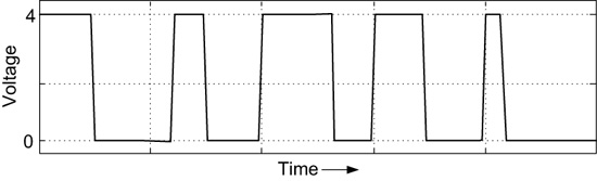
The second and more common definition of digital signal requires careful explanation. As an everyday example, when you look at a standard wall clock with its rotating minute and hour hands, the minute hand may point to the number 2 telling us it’s 10 minutes past the hour, as shown in Figure 4-2(a). Over the next 60 seconds, the minute hand slowly rotates to 11 minutes past the hour as shown in Figure 4-2(b). On a digital clock, however, at 10 minutes past the hour the minutes display will show the value 10. And for the next 59 seconds, the minutes display continues to show the number 10. Then all of a sudden, the digital clock’s minute display quickly switches to the number 11. Unlike a rotary-hand clock, a digital clock cannot show any time between 10 and 11 minutes past the hour. So, the minutes display on a digital clock is a digital number that can only be one of 60 possible whole numbers, either 00, 01, 02, 03, . . . , 58, or 59.
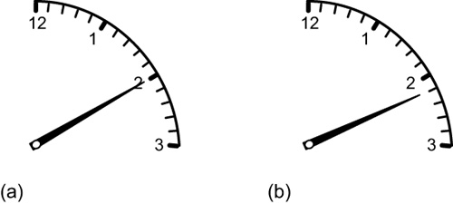
Figure 4-2 A rotary clock’s minute hand positions: (a) 10 minutes after the hour; (b) 11 minutes after the hour.
In a similar example, the typical automobile dashboard speedometer shows the car’s speed, in miles per hour (mph), as depicted in Figure 4-3(a). The speedometer’s pointer moves smoothly from left to right. However, some modern autos have digital speedometers that display an easy-to-read number, as shown in Figure 4-3(b). We are at liberty to call that number 48 in Figure 4-3(b) a digital number, as we did with the minutes display on a digital clock.
Figure 4-3 Automobile speedometer displays: (a) old-style analog pointer display; (b) digital display.
OK, let’s now consider a sequence of digital numbers. We start by recalling the low and high Marquette, Michigan, temperature curves in Figure 2–1. We repeat the low temperature curve here in Figure 4-4.
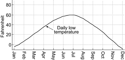
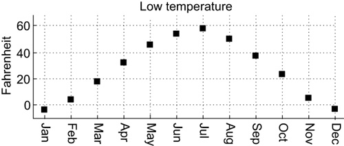
Instead of having the Figure 4-4 low temperature analog curve available to us, assume we have the following table of low temperatures obtained on the first day of each month over a period of one year.
If we plot Table 4.1’s sequence of 12 numbers as dots, one dot per number, we have the plot shown in Figure 4-5. That plot of dots is important because the list of temperature values in Table 4.1 is also called a digital signal and the plot in Figure 4-5 is a graphical depiction of this signal.

To establish our terminology here, we say the list of 12 numbers in Table 4.1 can be called:
• a digital signal (the least appropriate but by far the most common terminology),
• a digital sequence (occasionally used), or
• a discrete sequence (the most appropriate terminology but not commonly used).
We will comply with common terminology and state:
Digital signal definition #2: A sequence of discrete, individual numbers.
This is the definition we’ll use throughout the remainder of this book.
We turn now to the fundamental difference between the smoothly changing analog temperature signal in Figure 4-4 and the discrete, periodically spaced-in-time, digital temperature signal in Figure 4-5. Both signals tell us how the low outdoor temperature varies over a period of one year in Marquette, Michigan. Later, we’ll learn in what situations digital signals are more useful to us than are analog signals.
How Digital Signals Are Generated
There are three common methods used to generate digital signals. We discuss each method in the following paragraphs.
Digital Signal Generation by Observation
The digital signal in Figure 4-5 was obtained by observation. Over a year’s time, on the first day of the month, someone observed a thermometer and recorded the coldest temperature for that day. The observer then listed those 12 temperatures in Table 4.1. The digital signal, representing the physical quantity of temperature listed in Table 4.1, was obtained by observation.
Another example of a digital signal generated by observation is the daily closing prices of one share of Apple (Apple Inc.) stock. The prices, observed over a three-year period and measured in U.S. dollars, form a digital signal, a discrete sequence of numbers, as shown in Figure 4-6(a).
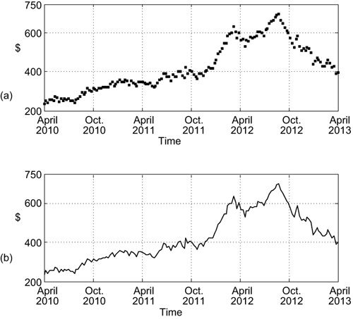
Figure 4-6 Closing price of one share of Apple stock: (a) daily prices plotted as dots; (b) preferred display method of connecting the dots with lines, and then deleting the dots.
Stock market analysts routinely record, compile, and examine historical daily stock prices like these. However, rather than plotting a sequence of prices as dots, similar to what we did in Figure 4-6(a), analysts connect the dots with lines and then delete the dots, producing a jagged curve as shown in Figure 4-6(b). Note that the curve in Figure 4-6(b) is not a continuous analog signal. It’s merely the popular way to graphically depict the digital data in Figure 4-6(a).
As for the information content of Figure 4-6, many readers will find that figure of little interest. However, for those readers who bought or sold shares of Apple Inc. stock during the summer of 2012, Figure 4-6 contains crucial information.
By the Way
Thanks to the Internet, you can examine the historical stock share prices of any company registered with any major stock exchange. You may want to visit this Web site, http://finance.yahoo.com, to check the historical and current stock price of your employer.
Digital Signal Generation by Software
Another way digital signals are generated is through the use of computer software. Engineers frequently use software to create digital signals needed for analysis or testing purposes. The results of their efforts are digital signals, lists of numbers stored in a computer’s memory that may represent any physical quantity of an engineer’s choice. In later chapters, we’ll look at several examples of software-generated digital signals.
Digital Signal Generation by Sampling an Analog Signal
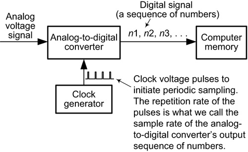
By far the most common way digital signals are generated is by sampling, a process by which we represent an analog signal with a list of numbers. The process of sampling is depicted in Figure 4-7. An analog voltage signal is applied to a small electronic device called an analog-to-digital converter. For convenience, we’ll refer to an analog-to-digital converter as an ADC. The output of the ADC is a sequence of numbers, n1, n2, n3, . . . , that is stored in a computer’s memory. The sequence of numbers is our digital signal obtained by sampling an analog voltage signal.

Figure 4-7 Sampling: converting an analog signal to a digital signal for storage in computer memory.
Critical to our sampling process are the periodically spaced clock voltage pulses applied to the ADC. Those pulses determine the exact instants in time when the converter will measure the analog voltage’s instantaneous value and generate a single output number representing that value. Let’s look at an example of sampling an analog voltage signal.
We show the input and output of a sampling process in Figure 4-8. Let’s assume the analog voltage input signal to an ADC is the sinusoidal voltage shown in Figure 4-8(a). As shown in that figure, we sample the analog ADC input voltage at the equally spaced instants in time represented by the vertical arrows.
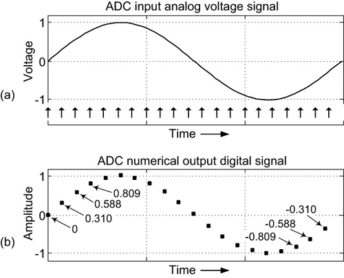
Figure 4-8 Analog-to-digital converter operation: (a) analog signal input; (b) digital signal output.
The sampled values, the sequence of 20 numbers output by the ADC, are listed in Table 4.2. Those sample values are also graphically depicted as dots in Figure 4-8(b). Each dot represents one sample value, one number, of the sampled sequence.
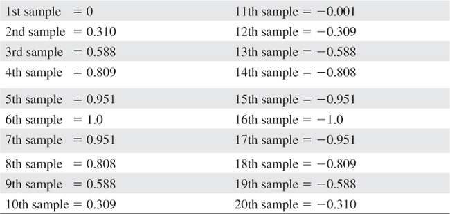
If we took it upon ourselves to draw the ADC output sequence on a piece of paper with time on the horizontal axis as in Figure 4-8(b), the tip of our pen or pencil would indeed leave the surface of the paper, unlike drawing a continuous analog signal.
The sequence of numbers in Table 4.2 comprises the ADC’s output digital signal, and those numbers can be stored in a computer’s memory. We refer to the ADC output sample values, the sequence numbers represented as dots in Figure 4-8(b), as a sampled version of the analog signal in Figure 4-8(a). So there you are. The sequence of numbers listed in Table 4.2, and represented by the dots in Figure 4-8(b), is a digital signal.
The Sample Rate of a Digital Signal
In the world of digital signal processing (DSP), every digital signal sequence of numbers has what is called a sample rate associated with it. The sample rate of a digital signal is the repetition rate of the signal’s samples, measured in samples per unit of time. And the sample rate of a digital signal is extraordinarily important. In Figure 4-7, the sample rate of the n1, n2, n3, . . . digital signal is the repetition rate (the frequency) of the clock signal used to initiate the conversion of the analog voltage signal. The notion of sample rate, how often an analog signal is sampled, is fairly easy to understand.
For example, if someone sent you an e-mail listing the 20 digital signal sample values in Table 4.2 and you created your own version of Figure 4-8(b), you’re missing an important piece of information. You would have no idea what the frequency is of the analog sine wave that was sampled to produce the digital signal in your drawing. Did the sine wave repeat every second, every 10 seconds, or once a week? On the other hand, if you knew what the sample rate of the e-mailed digital signal was, say 60 samples/second, you would then be able to step through the arithmetic and determine that:
• 60 samples spans 1 second of time,
• 20 samples spans 1 cycle of the analog sine wave,
• 20 samples is one-third of a second (20/60 = 1/3),
• 1 cycle of the analog signal lasts one-third of a second,
• 3 cycles of the analog sine wave last 1 second, and
• the frequency of the analog sine wave is 3 cycles/second, or 3 Hz.
Again, to fully understand the digital signal represented by the dots in Figure 4-8(b), we need to know the sample rate of that sequence of numbers.
To test your understanding of sample rate, we ask: what are the sample rates of the digital signals in Figure 4-5 and in Figure 4-6(a)? Hopefully, your answer is: the sample rate for the digital signal in Figure 4-5 is one sample per month and the sample rate for the digital signal in Figure 4-6(a) is one sample per day.
A Speech Digital Signal
Let’s now look at a slightly more complicated digital signal. In Chapter 2, we discussed an analog voltage representing the audio speech signal of Capt. Kirk speaking the words “Mister Spock.” We also looked, in greater detail, at the analog audio signal of the first syllable, “Mis,” of the word Mister. Figure 2-12(b) shows the details of the analog voltage waveform of the audio syllable “Mis.”
The sampled version of that analog audio “Mis” signal, a digital signal, is shown by the dots in Figure 4-9(a). As a digital signal, the syllable is more complicated than we would expect, as we see in Figure 4-9(a), where it looks like a dense jumble of dots. To help us understand the nature of the signal, we could connect the dots with straight lines as in Figure 4-9(b). However, this is only a slight improvement visually. For more visual clarity, DSP folks connect the dots in Figure 4-9(a) with lines and then delete the dots to obtain Figure 4-9(c). This simplified version shows the fluctuating amplitude of the digital signal so that it’s easier to visualize and understand. Yes, Figure 4-9(c) looks like an analog signal. But in looking at this sort of figure, DSP engineers realize that the figure represents a digital signal (a sequence of discrete numbers) rather than a continuous analog signal.
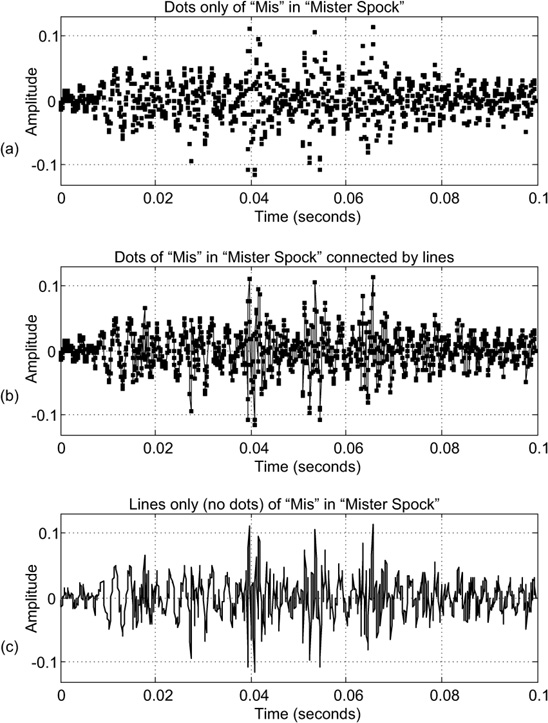
Figure 4-9 Displaying the digital speech signal, “Mis”: (a) samples plotted as dots; (b) dots connected by lines; (c) dots connected by lines and dots removed.
The sample rate of the Figure 4-9 digital speech signal is 11,025 samples/second. That sample rate might seem like a strange value but it’s a sample rate commonly used by audio signal processing engineers. Four times 11,025 is 44,100 samples/second, which is the industry standard sample rate used for recording the digital signals of music on compact discs (CDs). We have more to say about sample rates later in this chapter.
OK, to provide illustrations of why it’s beneficial to sample an analog audio signal to obtain a digital audio signal, let’s look at two simple examples of audio digital signal processing.
An Example of Digital Signal Processing
Let’s say we’re working in a music studio and a pop singer is recording a new song. And say that, unfortunately, during the third verse of the song the singer sings one note off-key. Decades ago, the entire song would have to be rerecorded to correct this. And, hopefully, the singer would sing the song perfectly on key during the second recording while maintaining the same emotional intensity as the first recording.
Nowadays, thanks to digital signal processing, correcting performance errors by rerecording entire songs is no longer necessary. Today, the singer’s analog voice signal can be sampled by an analog-to-digital converter, and then the digital signal samples are passed to a computer as shown in Figure 4-10. In that figure, the sequence of sampled values (numbers) making up the digital vocal signal are represented by the x1, x2, x3, . . . notation.
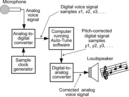
Now let’s assume the computer is running commercial software called Auto-Tune®. This software analyzes all the digital samples of the recording by measuring the pitch (frequency) of each musical note sung by the singer. If the software detects a note sung off-key (wrong pitch or frequency), the software determines the on-key note (correct pitch or frequency) that is nearest in pitch to the off-key note. Then, the software replaces the samples of the off-key note with samples of the on-key note.
For example, let’s say that the software encounters a sequence of samples of a vocalized note shown by the dots in Figure 4-11(a), and determines that the pitch (frequency) of that note is off-key based on the specified musical key of the song. Next, the software determines the nearest on-key note for that part of the song represented by the dashed-curve waveform in Figure 4-11(a). The software then replaces the off-key samples in Figure 4-11(a) with corrected samples shown in Figure 4-11(b), which represent the nearest on-key note. Notice how the corrected samples in 4-11(b) match the on-key waveform of the dashed curve in 4-11(a).
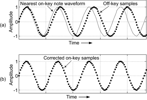
Figure 4-11 Correcting an off-key musical note: (a) samples of an off-key musical note (dots) and the nearest correct note’s waveform; (b) samples of the corrected on-key musical note.
The pitch-corrected y1, y2, y3, . . . digital signal samples of the entire song are then routed to a digital-to-analog converter, which transforms them into an analog signal as shown in Figure 4-10. (We discuss the operation of digital-to-analog converters in a later chapter.) When the analog signal is connected to a loudspeaker, we hear the singer’s voice with every musical note perfectly on-key.
This pitch-correction process is used not only in music studios for recording music CDs, but also in live performances in stadiums filled with screaming fans. This type of pitch correction would be impossible without modern digital signal processing.
By the Way
Auto-Tune software makes life easier for people in the music business. That’s the good news. The bad news is that you can never again listen to your favorite singer and know whether you’re listening to their natural voice or to their Auto-Tune-corrected voice. As it turns out, old vinyl albums with a famous artist occasionally singing off-key are often worth much more money than their corrected, re-mastered CD counterparts.
Another Example of Digital Signal Processing
To understand our second example of why sampling an analog audio signal to obtain a digital signal is beneficial, let’s consider how telephones worked in the mid-1900s.
Some of you might be old enough to remember the rotary-dial landline telephone shown in Figure 4-12. To place a call, the user had to lift the handset off the hook, insert a finger in the appropriate numbered hole in the round dial, and rotate the dial clockwise until it encountered a stop. When the user removed his or her finger, a rotary spring spun the dial back to its original position. As the dial spun counter clockwise, an electrical switch was closed and then opened multiple times sending electrical pulses to the telephone company’s switching station. (It was similar to quickly flicking a light switch on and off multiple times.) If you started your dialing from the number 4 hole in the dial, four electrical pulses were transmitted to the phone company. To make a local phone call you had to repeat this rotary dialing process six more times, once for each of the seven digits of the destination phone’s telephone number.
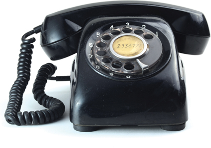
At the telephone company’s switching station, electrical hardware would interpret the seven sets of electrical pulses (seven pulses for each number dialed) and automatically, using relay switches, electrically connect your telephone’s wires to the destination telephone’s wires. For technical reasons, using the early rotary-dial telephones required telephone company operator assistance to make long-distance calls. (Your grandparents well remember the phrase, “Number please.”) Be that as it may, the rotary-dial telephone was a great innovation. It eliminated the need for operator assistance for local phone calls.
But technology marched on. Thanks to digital signal processing, making telephone calls became even easier in the early 1960s with the innovation known as the touch-tone telephone that we use today. Modern telephones have a rectangular keypad, shown in Figure 4-13, that we use to make phone calls.
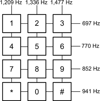
On touch-tone phones, pushing a key activates two internal audio oscillators to generate two distinct analog audio tones whose frequencies depend on which key was pushed. For example, pushing the 8 key generates an 852 Hz audio tone and a 1,336 Hz audio tone that are added together to produce a composite analog audio signal. Likewise, pushing the 4 key generates a 770 Hz audio tone and a 1,209 Hz audio tone that are added together to create a composite analog voltage signal, as shown on the right side in Figure 4-14. That composite analog voltage is transmitted over telephone wires to the telephone company’s switching station.
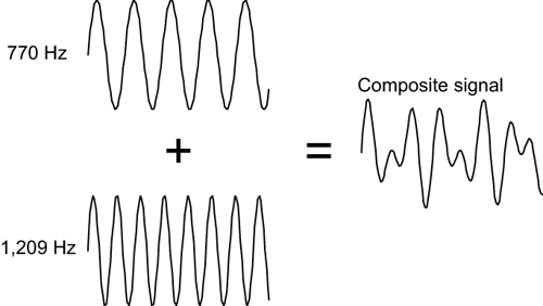
Figure 4-14 Composite audio signal (a 770 Hz tone plus a 1,209 Hz tone) generated when the 4 key is pressed on a touch-tone telephone keypad.
When the Figure 4-14 composite analog signal arrives at the telephone company switching station, it is sampled by an analog-to-digital converter to generate the digital signal samples represented by the dots in 4-15(b).
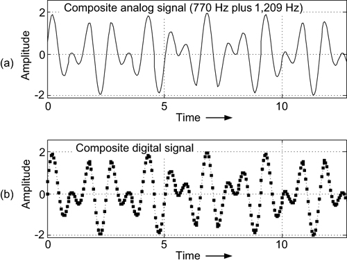
Figure 4-15 Composite audio signal created when the 4 key on a touch-tone telephone’s keypad is pressed: (a) analog signal sent to the telephone company; (b) digital signal generated, by sampling, at the telephone company.
That process of analog-to-digital conversion is shown in Figure 4-16. The digital samples are subsequently routed to electronic hardware that performs digital signal processing operations to recognize the frequencies of the two tones contained in the composite signal. This determines which key the telephone caller pressed. The digital signal processing implements an array of tone detectors as shown in Figure 4-16. If the caller presses the telephone’s 4 key, the 770 Hz and 1,209 Hz detectors’ outputs are activated and the system determines that, indeed, the 4 key was pressed.
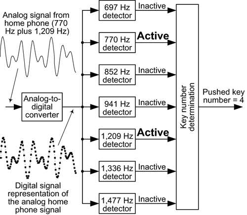
Figure 4-16 Touch-tone telephone pushbutton key recognition process at the telephone company’s switching station when the 4 key is pressed.
So what are the big deals about a touch-tone home telephone and the digital signal processing that takes place in the telephone company’s switching station? The big deals are:
• At the switching station, the hardware to detect digital audio tones is significantly smaller in size, less expensive, more reliable, faster, and more power efficient than the hardware used to detect old-style, rotary-dial telephone pulses.
• Your touch-tone home phone is smaller in size, lighter in weight, less expensive, and faster in operation than the old-style rotary phones. In addition, no telephone operator assistance is needed for long-distance calls when using touch-tone home phones.
By the Way
Digital telephone signals are sometimes relayed by orbiting satellites where the signal is received and then relayed to another continent using high-power on-board amplifiers. These satellites are about 23,000 miles above the equator. Even at the speed of light, it takes about one-quarter of a second (called satellite latency) for the signal’s round trip. You notice this on newscasts when the reporter on foreign soil seems to delay his or her answer to a question from the network studio. It’s also noticeable in international personal phone calls when you ask, “Do you miss me?” and your sweetheart seems to hesitate before answering!
Two Important Aspects of Sampling Analog Signals
There are two additional important topics related to sampling an analog signal to generate its corresponding digital signal. We cover these in depth in subsequent chapters, but introduce them briefly here. The first topic is a fundamental restriction imposed on the sample rate used in the analog-to-digital conversion process. The second is the precise characteristics of the numbers produced at the output of an analog-to-digital converter. Let’s briefly consider those two topics.
Sample Rate Restriction
As we stated earlier, when we sample an analog signal to generate its corresponding digital signal, as shown in Figure 4-17, we must apply clock voltage pulses to the analog-to-digital converter. The repetition rate of those voltage pulses, measured in samples per second, is called the sample rate (or sample frequency) of our sampling process. For example, the sample rate of the Figure 4-9 digital speech signal is 11,025 samples/second.
To ensure that the digital signal sequence of numbers, n1, n2, n3, . . . , accurately represents the input analog signal, the sample rate (sampling frequency) of an analog-to-digital converter’s clock signal must be greater than twice the frequency of the highest-frequency spectral content of the input analog signal. In the field of digital signal processing, this is called the Nyquist sampling criterion. For example, the sample rate of 11,025 samples per second for the digital speech signal in Figure 4-9 is well above twice the highest frequency content of normal conversation.
The origin of this criterion and the ill effects of violating it are so important in the world of digital signal processing that we’ve dedicated the next chapter, titled “Sampling and the Spectra of Digital Signals,” to these topics.
Analog-to-Digital Converter Output Numbers
The second important topic regarding the process of sampling an analog signal is the nature of the numbers produced by an analog-to-digital converter.
When we sample an analog signal, as shown in Figure 4-17, the digital signal’s sequence of numbers is not in the form of decimal numbers that we’re so familiar with in our daily lives. The digital signal’s sequence of numbers, n1, n2, n3, . . . , are in the form of what we call binary numbers. The interesting topics of binary numbers and why we use them are discussed in Chapter 9.
Sample Rate Conversion
When reading the literature of digital signal processing or listening to signal processing engineers, you may encounter the terms decimation and interpolation. Those terms refer to changing the sample rate of a digital signal.
That might seem like a strange idea but changing the sample rate of a digital signal, known as sample rate conversion, has many applications. In fact, both decimation and interpolation take place whenever you use your cell phone or smartphone. In the following sections, we briefly describe the processes of both decimation and interpolation.
Decimation
Regardless of its dictionary definition, for us the term decimation means to reduce the sample rate of a digital signal. We’ll explain this idea with an example.
Consider the 250 Hz sine wave voltage signal shown in Figure 4-18(a). If we sampled that analog signal using an analog-to-digital converter, at a sample rate of 3,000 Hz the resulting digital signal’s samples would be those shown in Figure 4-18(b). If, for some reason, we wanted a digital version of the original analog signal having a sample rate of 1,000 Hz, we would not need to repeat an analog-to-digital conversion process. We could simply decimate the Figure 4-18(b) digital signal by a factor of 3. That decimation-by-3 process means we simply retain every third sample of the Figure 4-18(b) signal, and discard the remaining samples. Retaining only every third sample of the Figure 4-18(b) signal results in our desired 1,000 sample rate digital signal shown in Figure 4-18(c).
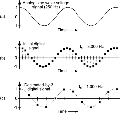
Figure 4-18 Decimation by a factor of 3: (a) original 250 Hz analog sine wave voltage signal; (b) initial digital signal having a sample rate of 3000 Hz; (c) decimated-by-3 digital signal having a sample rate of 1,000 Hz.
Interpolation
Interpolation refers to the process of increasing the sample rate of a digital signal. As we did with decimation, let’s look at that idea by way of an example.
Figure 4-19(a) shows a digital signal whose sample rate is 1,000 Hz. Suppose we want that signal to have a sample rate of 3,000 Hz (higher-frequency sampling rate). The first step in our interpolation-by-3 process is to create a modified digital signal by inserting two zero-valued samples in between each of the original digital signal’s samples. That new digital signal is shown in Figure 4-19(b), where the zero-valued samples are represented by the circular dots. The sample rate of the Figure 4-19(b) signal is now 3,000 Hz as indicated in Figure 4-19(c). Our final step is to pass the Figure 4-19(b) signal through a digital lowpass filter whose output signal is our desired interpolated-by-3 signal shown in Figure 4-19(d). A lowpass filter is a process that allows low-frequency signal energy to pass, but blocks high-frequency signal energy. We discuss the behavior and implementation of digital lowpass filters in Chapter 8.
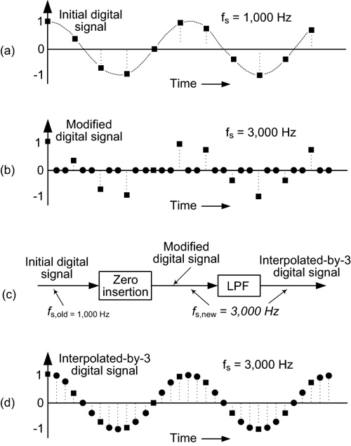
Figure 4-19 Interpolation by a factor of 3: (a) original digital signal having a sample rate of 1,000 Hz; (b) modified digital signal with zero-valued samples inserted; (c) interpolation process signal flow; (d) interpolated-by-3 digital signal having a sample rate of 3,000 Hz.
Where decimation by 3 was a single-step process of simply discarding time samples, interpolation by 3 is a two-step process of zero-valued sample insertion followed by lowpass filtering.
• The phrase digital signal has two different meanings:
– Definition #1: An analog voltage signal that alternates between two distinct voltage values (see Figure 4-1).
– Definition #2: A sequence of discrete, individual, numbers (see Figure 4-5.)
We use definition #2 in this book.
• Digital signals, discrete sequences of numbers, can be stored in the memory of a computer.
• Digital signals are produced in three ways:
– Observing and collecting meaningful data (see Figure 4-6(a))
– Computer software
– Sampling an analog signal using analog-to-digital converter hardware (see Figure 4-7 and Figure 4-8)
• Digital signals have a sample rate associated with them. The sample rate of a digital signal is the repetition rate of the signal’s samples measured in samples per unit of time. For example, the sample rate for the digital signal in Figure 4-5 is one sample per month. The sample rate for the digital signal in Figure 4-6(a) is one sample per day. The sample rate for the digital signal in Figure 4-9(a) is 11,025 samples per second.
• To ensure that a digital signal sequence accurately represents an analog signal, the sample rate (sampling frequency) of an analog-to-digital converter’s clock signal must be greater than twice the frequency of the highest-frequency spectral content of the analog signal.
• The term decimation refers to the process of decreasing the sample rate of a digital signal. The term interpolation refers to the process of increasing the sample rate of a digital signal.