B. Decibels
Signal processing engineers often need to measure the amplitude difference between two signals. For example, an engineer might need to compare the amplitude of a signal at the output of an amplifier to the amplitude of that signal at the input of the amplifier. Comparing the amplitude of those two signals describes the gain (the amount of amplification) of the amplifier. In practice, however, because various signals have such a wide range of amplitude values to be compared, engineers find it convenient to use decibels to simplify their numerical comparisons. This appendix describes how this is done.
The use of decibels is an expedient mathematical method for comparing the amplitude, or power, difference between two signals or between any two natural phenomena. That may sound a bit mysterious, but there’s a good chance you’re already familiar with use of decibels. We’ll cover two examples of decibels that you are already acquainted with and then discuss decibels as they’re used in signal processing.
Before we remind you of decibel values that you’ve encountered before, we simply must present one form of the equation for computing decibel values used to compare two numbers. That equation is:
We use the letters dB to represent the word decibels, much like we use the letters mph to represent the words miles per hour.
Don’t be troubled by equation (B-1). (We won’t ask you to compute any decibel values; we’ll do any of the necessary calculations for you.) Stated in words rather than numbers, equation (B-1) is “the decibel value of number P1 compared to number P2 is 10 times the base-10 logarithm of the fraction P1 divided by P2.” OK, with that said, let’s look at a use of decibels that you’ve encountered in your daily life.
Decibels Used to Describe Sound Power Values
Acoustic engineers, and some health officials, are concerned with measuring the power of audio sounds to which people may be exposed. And because the range of power (the loudness) of various sounds we might be subjected to in our daily lives is so large, decibels are used by technical people to categorize the power of those sounds. It’s quite possible that, at one time or another, you have encountered the sound power values listed in the third column of Table B.1.
Acoustic engineers use their audio test equipment to measure the sound power value (in watts) in a particular environment, and declare that power value as number P1 in equation (B-1). By mutual agreement in the audio engineering field, the value of 0.000000000001 watts (10-12 W) is defined as the number P2. (See Appendix A for an explanation of that 10-12 notation.) Then, numbers P1 and P2 are inserted in equation (B-1) to compute a sound value measured in dB, such as the values in the third column of Table B.1. Again, decibels are used because it’s easier to discuss, interpret, and document the simpler dB values than the clumsy, wide-ranging center-column wattage numbers in Table B.1.
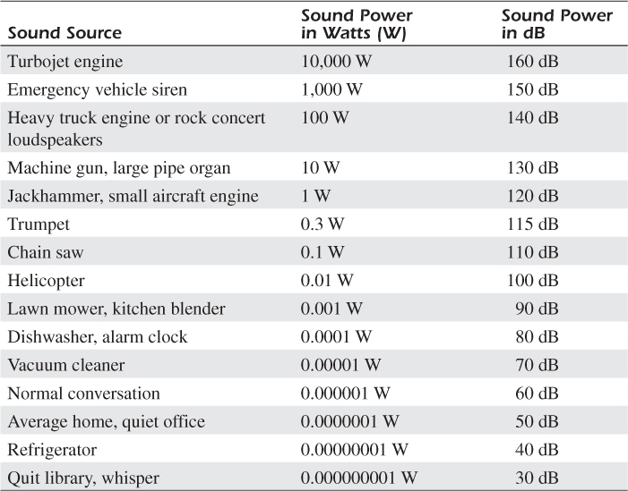
The main thing to notice in Table B.1 is that a difference of 10 dB, in the rightmost column, means a sound power difference factor of 10. This means that a difference of 20 dB is a sound power difference by a factor of 100. So standing near a running lawn mower (90 dB) is 100 times louder than standing near a running vacuum cleaner (70 dB).
By the Way
In the early twentieth century, signal processing people compared the power of two signals using the equation
log10(P1/P2) bels
where the unit bel was named in honor of the American inventor of the telephone, Alexander Graham Bell. The unit of bel was soon found to be inconveniently large. For example, it was discovered that the human ear could detect audio power value differences of one-tenth of a bel. Measured power value differences smaller than one bel were so common that it led to the use of the decibel (bel/10), effectively making the unit of bel obsolete.
Let’s look at another common use of decibels that may be familiar to you.
Decibels Used to Measure Earthquakes
When you hear in the news of an earthquake that has happened somewhere on our planet, you’re likely to hear the total energy of that earthquake specified by a value on what’s called the Richter scale. Seismologists also use a logarithmic equation to compute Richter scale values, similar to our sound power values in dB. That Richter scale equation is
We need not worry about the meaning of the energy values E1 and E2 in equation (B-2). We presented equation (B-2) merely to show that the mathematical operation of logarithms is used to categorize earthquake energies in the same way logarithms were used to compute sound power values in equation (B-1) and Table B.1.
Table B.2 presents a list of common Richter scale values for earthquakes. The center column of the table gives an estimate of an earthquake’s total energy in terms of the equivalent explosive energy of tons of TNT (similar to dynamite).
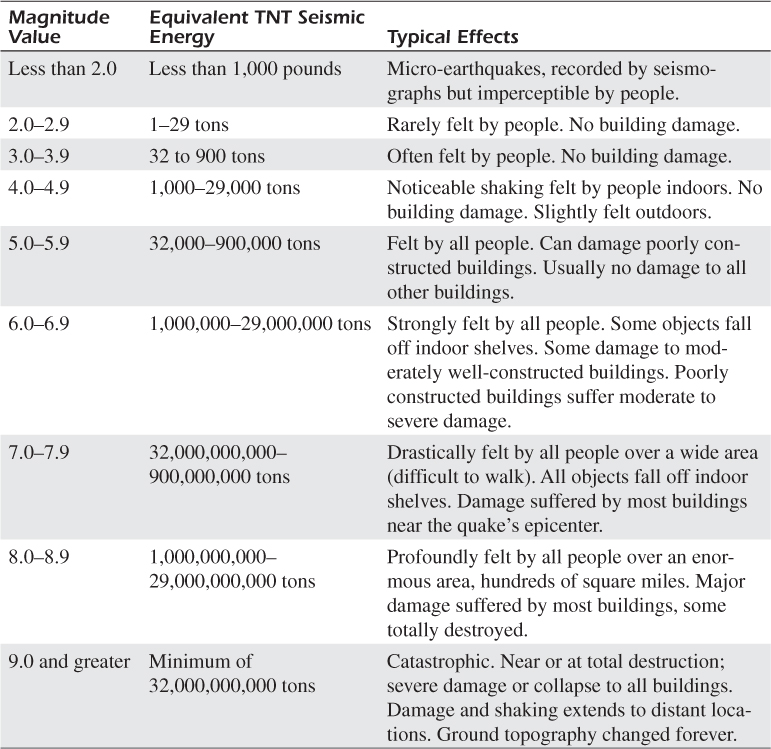
The main thing to notice in Table B.2 is that a Richter value difference of 1, in the leftmost column, means an energy difference factor of 10. This means that a Richter scale difference of 2 is an energy difference by a factor of 100. So an 8.0 earthquake is 100 times as destructive as a 6.0 earthquake.
Similar to Table B.1’s decibel (dB) sound power level values, it’s easier to discuss, interpret, and document Table B.2’s Richter scale values than the clumsy wide-ranging center column TNT energy values.
OK, now that we’re familiar with converting wide-ranging numbers to simpler smaller-ranging numbers, let’s see how signal processing engineers perform that same conversion.
Decibels Used to Describe Signal Amplitudes
As we stated at the beginning of this appendix, signal processing engineers use decibel values to conveniently compare the voltage amplitude levels of two signals. Similar to equations (B-1) and (B-2), signal processing folk use the equation
to compute a decibel (dB) value that represents the relative amplitude difference between two signals. Value A1 is the voltage amplitude of one signal and value A2 is the voltage amplitude of the other signal that we’re comparing to signal A1. Before we look at an example of using decibels in signal processing, we present Table B.3 showing the relationship between the ratio of two signal amplitudes and equivalent decibel values. Spend a few moments reviewing Table B.3. Notice that when A1 is less than A2, ratio A1/A2 is less than 1, and the dB value is a negative number.
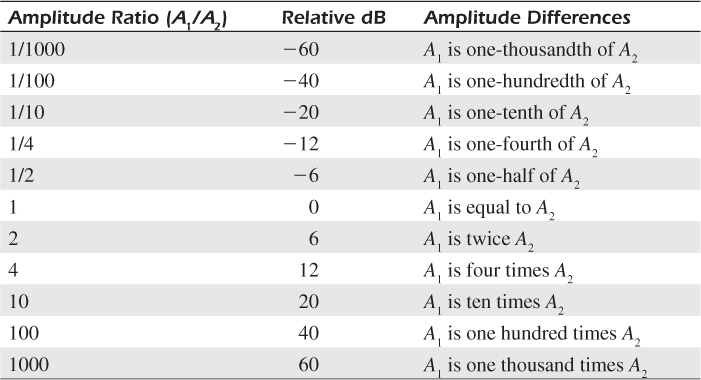
For example, here’s how we interpret Table B.3: if the voltage amplitude of signal A1 is one-tenth of the voltage amplitude of signal A2, we say “the amplitude of A1 is minus 20 dB relative to signal A2.” Signal processing engineers often speak in the language of dB.
As with the previous tables in this appendix, it’s easier to discuss, interpret, and document Table B.3’s center column dB values than the clumsy, wide-ranging amplitude ratios in the left column.
OK, let’s now look at a simple example of using decibels in signal processing that illustrates the dB values in Table B.3. Figure B-1(a) shows a composite analog signal. We will call that signal by the name Sin. Signal Sin is the sum of a 2 kHz sinusoidal wave whose positive peak amplitude is 1, and a 3 kHz sinusoidal wave whose positive peak amplitude is 0.8. For illustrative purposes, we show the individual 2 kHz and 3 kHz sinusoidal waves in Figure B-1(b). Again, the Figure B-1(a) Sin signal is the sum of the solid- and dashed-line waves in Figure B-1(b). The spectrum of signal Sin is given in Figure B-1(c).
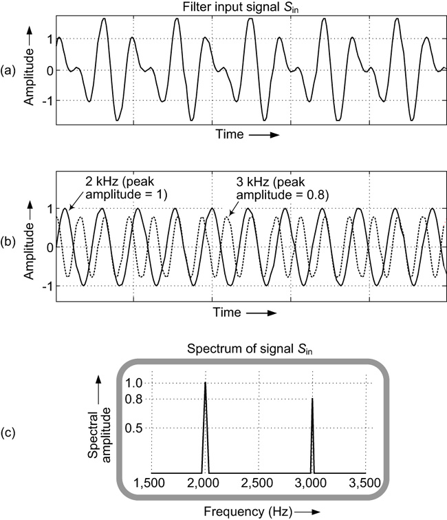
Figure B-1 Analog signal:(a) composite time signal Sin; (b) individual 2 kHz and 3 kHz time signals; (c) individual 2 kHz and 3 kHz spectral components.
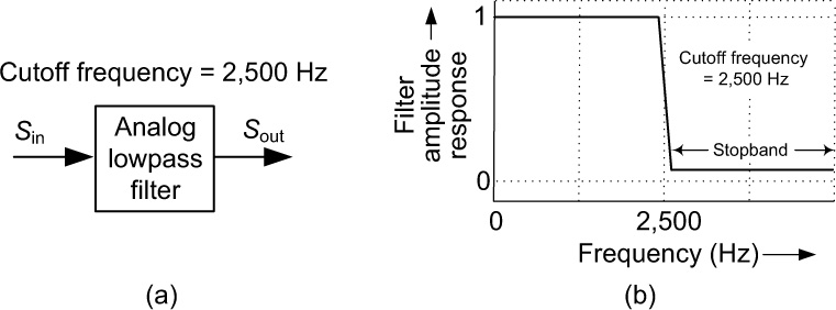
Let’s assume we decide to remove (filter out) the 3 kHz component from the composite Sin signal. We can do that by passing signal Sin through the lowpass filter shown in Figure B-2(a). The lowpass filter, whose cutoff frequency is 2,500 Hz, operates as follows: any filter input-signal spectral energy with a frequency less than 2,500 Hz will pass through the filter and show up at the filter’s output with no loss in amplitude. In addition, any filter input-signal spectral energy with a frequency greater than 2,500 Hz will pass through the filter and show up at the filter’s output but with a significant loss in amplitude. That behavior is shown in Figure B-2(b).
Passing the Figure B-1(a) Sin signal through the lowpass filter produces an Sout output signal shown in Figure B-2(a), which looks like the 2 kHz solid-line curve in Figure B-1(b). It appears that the lowpass filter has eliminated the 3 kHz component. But how well did our filter really work? Let’s say we apply the Sout signal to the input of a spectrum analyzer and obtain the display given in Figure B-3(b). There, we see that Sout still contains a very small amount of the 3 kHz sine wave. Using decibels, we can specify exactly to what degree our lowpass filter attenuated the undesired 3 kHz sine wave. Here’s how.
From Figure B-1(c), the amplitude of the 3 kHz component of signal Sin at the filter’s input is 0.8. We assign that amplitude value to the variable A2 in equation (B-3). From Figure B-3(b), the amplitude of the undesired 3 kHz component of signal Sout at the filter’s output is 0.008, so we assign that amplitude value to the variable A1. The ratio A1/A2 now becomes A1/A2 = 0.008/0.8 = 0.01 = 1/100. From Table B.3, an A1/A2 ratio of 1/100 is equivalent to –40 decibels (dB). So there you have it. We can now describe the filter’s performance in either of these two equivalent ways:
• The lowpass filter’s stopband gain is –40 decibels (–40 dB).
• The lowpass filter attenuated signal Sin’s undesired 3 kHz component by 40 dB.
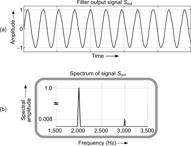
Figure B-3 Lowpass filtering:(a) individual 2 kHz and 3 kHz output spectral components; (b) output time signal Sout.
On the off chance that you ever need to compute the relative dB difference between the amplitudes of two signals using equation (B-3), you don’t necessarily need a scientific hand calculator. You can compute dB values using Microsoft Excel spreadsheet software. For example, to compute the decibel level of an amplitude of 0.008 divided by an amplitude of 0.8, in a cell of an Excel spreadsheet merely enter the following:
=20*LOG10(0.008/0.8)
Then hit your keyboard’s Enter key. The number –40 will appear in that cell, meaning a decibel value of –40 dB.
Decibels Used to Describe Filters
Decibel values are very often used to describe the performance of both analog and digital filters. Using equation (B-3), signal processing engineers plot a curve of a filter’s frequency-domain behavior where the vertical axis is measured in decibels. An example of this, for a bandpass filter, is shown in Figure B-4.
Recall the lowpass filter in Figure B-2 that only allowed signals whose frequencies were greater than 2,500 Hz to pass through the filter. Figure B-4 is a bandpass filter that allows signals whose frequencies are within a frequency band to pass through the filter.
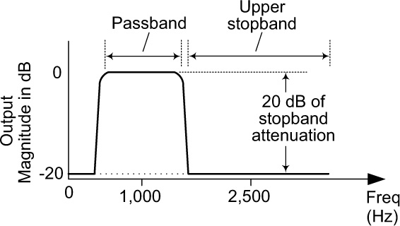
We interpret Figure B-4 as follows: Let’s say we apply a 1,000 Hz sine wave, whose amplitude is A2, to the input of the bandpass filter. According to Figure B-4, the A1 amplitude of the 1,000 Hz filter output sine wave is zero decibels (dB) relative to the A2 input amplitude. From Table B.3, we see that zero dB means that the ratio A1/A2 is equal to 1. So the 1,000 Hz output sine wave’s amplitude is equal to the 1,000 Hz input sine wave’s amplitude. The input 1,000 Hz sine wave arrived at the filter output with no reduction (no attenuation) in amplitude.
On the other hand, assume we now apply a 2,500 Hz sine wave, whose amplitude is A2, to the input of the bandpass filter. According to Figure B-4, the A1 amplitude of the 2,500 Hz filter output sine wave is –20 decibels (–20 dB) relative to the A2 input amplitude. From Table B.3 we see that –20 dB means that the ratio A1/A2 is equal to 1/10. So the 2,500 Hz output sine wave’s amplitude is equal to the 2,500 Hz input sine wave’s amplitude divided by 10 (attenuated by a factor of 10).