3. Frequency and the Spectra of Analog Signals
In the last chapter, we looked at graphical plots of how analog signals vary in value (fluctuate) as time passes. Those plots are crucial in understanding the nature of any given analog signal. However, there’s another very useful, and revealing, way to describe an analog signal. That alternate description is called the spectrum of an analog signal. Although you don’t often encounter the concept of spectra in your everyday life, signal processing people study and analyze signal spectra every day. When engineers examine (analyze) an analog signal, knowing a signal’s spectrum is as important as knowing the temperature, blood pressure, and heart rate of a patient being examined by a medical doctor.
So, in our study of signal processing, it’s important that we learn what a signal’s spectrum is and why such information is useful. That’s the goal of this chapter. But before we discuss just what the spectrum of an analog signal is, we must, by necessity, briefly return to and focus on the notion of frequency.
Frequency
In the last chapter, we introduced the term frequency, a term that we now need to define in a more formal way.
Frequency is a characteristic of periodic (repetitive) events. For us, frequency is the measure of how often some repetitive event occurs over some period of time. That is, frequency is a number of cycles (repetitions) per some unit of time. For example, when the needle of the tachometer on an automobile dashboard points to the number 2, that means the automobile’s engine is rotating at a repetition rate of 2,000 revolutions per minute (RPM). Each revolution is a repetition, making the frequency 2,000 repetitions per minute.
Cycles per Second
In the last chapter, we discussed the idea of pinging a tuning fork and the fork’s oscillating sound wave arriving at a microphone. If the microphone’s output cable were connected to the input port of an oscilloscope, then the scope’s display would show the sinusoidal voltage signal depicted in Figure 3-1. For example, a tuning fork can be used to define the standard pitch of the A key on a piano keyboard (the A key above middle C). This standard pitch is called “A440.” Thus, in Figure 3-1 the frequency of those sinusoidal analog wave oscillations is 440 hertz (440 oscillations per second, 440 cycles per second). For brevity, engineers write 440 hertz as 440 Hz.
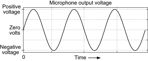
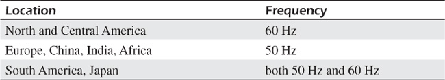
Another frequency you’re probably familiar with is the frequency of the AC (alternating current) electrical power at a wall socket in your home. Depending on your geographical location, the AC power line frequency will be either 50 Hz or 60 Hz. For example, in the United States, if you look at the bottom panel of any appliance on your kitchen counter, you’ll see the characters “60 Hz.”
A short list of power line frequencies is given in Table 3.1. AC power line voltages are sinusoidal in shape, meaning that the voltage of the hot conductor relative to the neutral conductor fluctuates from positive to negative, and then back to positive, just as does the voltage waveform in Figure 3-1.
In the early days of electricity, the unit of measure for frequency was cycles per second (cycles/second). That’s why the words “kilocycles/second” and “megacycles/second” are printed on the tuning dials of old radios to indicate frequency. In the 1960s, the European and North American scientific communities adopted the word hertz(Hz) as the unit of measure for frequency in honor of the German physicist, Heinrich Hertz, who first demonstrated radio wave transmission and reception in 1887.
The single-syllable word hertz was a good choice because it’s easy to say and it sounds plural in English. We’re fortunate that Hertz’s last name was nothing like Arnold Schwarzenegger’s.
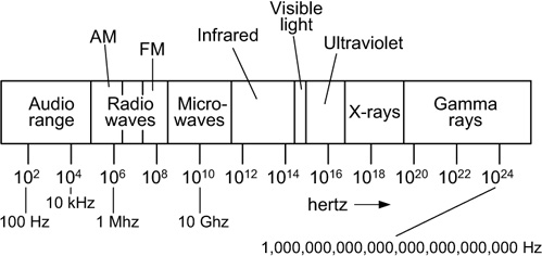
Signal processing engineers work with signals that cover an astounding range of frequencies. Audio engineers process analog signals in the frequency range of 20 Hz to 20 kilohertz (20 kHz, 20,000 Hz). Radio communications engineers deal with analog radio waves with frequencies in the range of kilohertz up to thousands of megahertz. Some cell phones operate at 900 megahertz. The frequency of the radiation inside the typical microwave oven is roughly 2.5 gigahertz (2,500 megahertz). Astronomers monitor analog stellar radiation with frequencies measured in terahertz (trillions of hertz). Table 3.2 gives the language and notation, and Figure 3-2 presents a crude graphical depiction, of various frequencies encountered in modern technology.
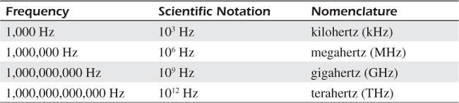
In case you haven’t seen it before, the notation in the center column of Table 3.2 is called scientific notation, a convenient and precise way for engineers and scientists to write very large and very small numbers. A review of that method for writing large numbers is provided in Appendix A.
Incidentally, the lowercase “k” in kHz is not a typographical error. For many decades, kilohertz has been abbreviated as kHz and megahertz has been abbreviated MHz with the uppercase “M.” That’s just the way it is.
Radians per Second
Occasionally you’ll hear an engineer refer to a sine wave’s or a cosine wave’s frequency in terms of radians per second. It’s straightforward to explain why people sometimes use such terminology.
Maybe you remember from geometry that the length of the circumference (perimeter) of a circle is π (pi) times its diameter.1 Since the diameter is twice the radius, the circumference of a circle can also be expressed as 2π times the radius length. To travel once around a circle takes 360 degrees, as shown in Figure 3-3(a). Likewise, to go once around the circle takes 2π radians, sometimes abbreviated as just 2π. So 360 degrees (one cycle) is equal to 2π radians. Therefore, a radian is an angle equal to 360°/2π, roughly 57.3°, as shown in Figure 3-3(b).
1. π = 3.14159 . . . is one of the fundamental constants in our universe. Its decimal digits extend to infinity to the right of its decimal point. But for us, we’ll just say that π = 3.14.
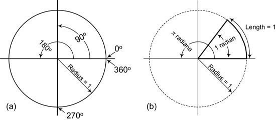
Again, from geometry we think of a circle as containing 360 degrees, but in their mathematical equations it’s much more convenient for engineers to think of a circle as containing 2π radians. In any case, if an engineer says a “sine wave’s frequency is 6280 radians/second,” that’s Geek Speak for 6280/2π = 1,000 Hz (cycles per second).
The Concept of Spectrum
So far in this chapter and in Chapter 2, we’ve looked at graphical representations of a few different fluctuating analog signals. We viewed two-dimensional graphs where the vertical axis of a graph represents a signal’s instantaneous amplitude (energy) and the horizontal axis represents time, as we saw in Figure 3-1. Such graphs, which show how a signal’s voltage amplitude level changes as time passes, are called time-domain plots. The horizontal axis of time-domain plots is always in units of time. Another powerful, and important, way to characterize analog signals is to describe their frequency content. The frequency content of a signal is called the signal’s spectrum.
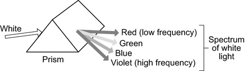
For us, the spectrum of a signal means the combination of sinusoidal waves of different frequencies that make up a signal. For example, you’re already somewhat familiar with the notion of a spectrum. If you shine a beam of white light on one side of a glass prism, multicolored light exits the opposite side of the prism as shown by the crude diagram in Figure 3-4. That’s because light changes direction when it moves from one medium (air) to another medium (glass). That direction change is called refraction, and the amount of refraction depends on the frequency of the light. So a prism can be used to break light up into its constituent spectral colors. Figure 3-4 shows us that white light is, in fact, a combination of multiple colors of light.
When you see a rainbow in the sky, water droplets in the atmosphere are behaving as individual prisms. The rainbow is caused by light being refracted while entering a droplet of water, then reflected from the back side of the droplet, and refracted again when leaving the droplet. If you’re lucky enough to ever see a double rainbow, the second rainbow is caused by light reflecting twice inside water droplets. The neat thing about double rainbows is that the sequence of colors in the secondary rainbow is reversed from the order of the colors in the primary rainbow.
Analog Signal Spectra
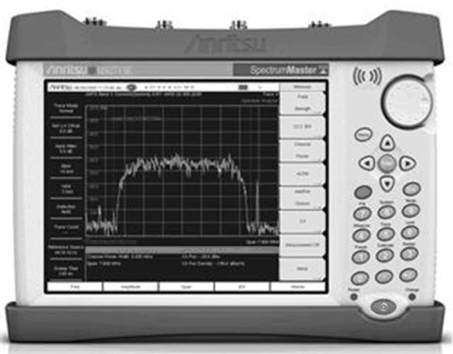
With this concept of spectrum in mind, engineers can actually display and measure an analog signal’s spectrum using a spectrum analyzer like that shown in Figure 3-5. A spectrum analyzer displays the combination of sinusoidal waves of different frequencies that make up an analog signal. Let’s look at a few examples of the spectra of analog voltage signals.
Assume a microphone’s output voltage is a 100 Hz sine wave as shown in Figure 3-6(a). Connecting that voltage to the input port of a spectrum analyzer would result in the analyzer’s frequency-domain display, which is shown in Figure 3-6(b). The horizontal axis of frequency domain plots is always in units of frequency, typically Hz. The front panel controls of the analyzer are set so that the start frequency and the stop frequency of the analyzer’s frequency display are 90 Hz and 110 Hz respectively.
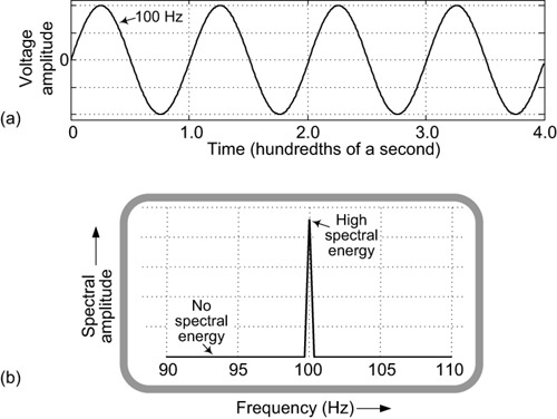
The spectrum analyzer contains a tuned-frequency energy detector that is initially tuned to the start frequency of 90 Hz. At that frequency, the analyzer detects no energy at its input that oscillates at 90 Hz, so at the horizontal position of 90 Hz on its display screen, the analyzer shows no spectral energy. The tuned-frequency detector is then tuned to 91 Hz where it detects no input 91 Hz spectral energy and, again at the horizontal position of 91 Hz on its display screen, the analyzer shows no spectral energy. The same thing happens as the tuned detector is tuned from 92 Hz up to 99 Hz. Then, when tuned to 100 Hz, the energy detector indicates a high level of input energy that oscillates at 100 Hz (100 cycles/second). That event causes the analyzer to display the high-level vertical spike at a frequency value of 100 Hz in Figure 3-6(b).
The analyzer’s tuned-frequency detector is subsequently tuned, in turn, from 101 Hz to the stop frequency of 110 Hz where, in each case, no spectral energy is detected and the analyzer’s display shows no input spectral energy in the frequency range of 101 to 110 Hz in Figure 3-6(b). That lone vertical spike in Figure 3-6(b) tells us that the voltage at the input of the spectrum analyzer contains a waveform oscillating at 100 Hz as we would expect by referring back to Figure 3-6(a).
Let’s say an engineer wants to actually verify the frequency of the microphone’s output sine wave voltage. There are two ways to do so. In the first method, the engineer could look at the voltage’s time waveform using an oscilloscope, mentioned earlier, to see the display in Figure 3-6(a). Measuring the time duration of one oscillation to be one hundredth of a second, the engineer then knows that 100 oscillations occur over a time interval of one second. Thus, the sine wave’s frequency is 100 Hz (100 cycles/second).
The second frequency measurement method is simpler. The engineer merely connects the sine wave voltage to the input of a spectrum analyzer, views the spectral display in Figure 3-6(b) to see the frequency location of the high-level spectral amplitude spike, and quickly determines that the sine wave’s frequency is indeed 100 Hz.
The point is that engineers sometimes look at analog signals’ amplitude waveforms over time using an oscilloscope, and sometimes they look at the spectral (frequency) content of analog signals, irrespective of time, using a spectrum analyzer. Spectrum analyzers are very powerful test instruments because their start and stop frequencies can be set to any values from tens of Hz to several GHz. An oscilloscope and a spectrum analyzer are as useful to engineers as a hammer and a saw are useful to carpenters.
With a spectrum analyzer, we could ping (vibrate) a tuning fork that has a tuned frequency unknown to us, near a microphone with its output cable connected to the input of a spectrum analyzer. Then, we could determine the tuned frequency of the tuning fork by observing the horizontal frequency location of the narrow spectral amplitude spike on the analyzer’s display. Neat, huh?
A Composite-Signal Spectral Example
To strengthen our understanding of signal spectra, consider the high-amplitude 100 Hz sine wave represented by the dashed-line curve in Figure 3-7(a). The figure also has a lower-amplitude 200 Hz sine wave shown by the dotted-line curve. (Notice how the 200 Hz sine wave oscillates twice for each complete oscillation of the 100 Hz sine wave.)
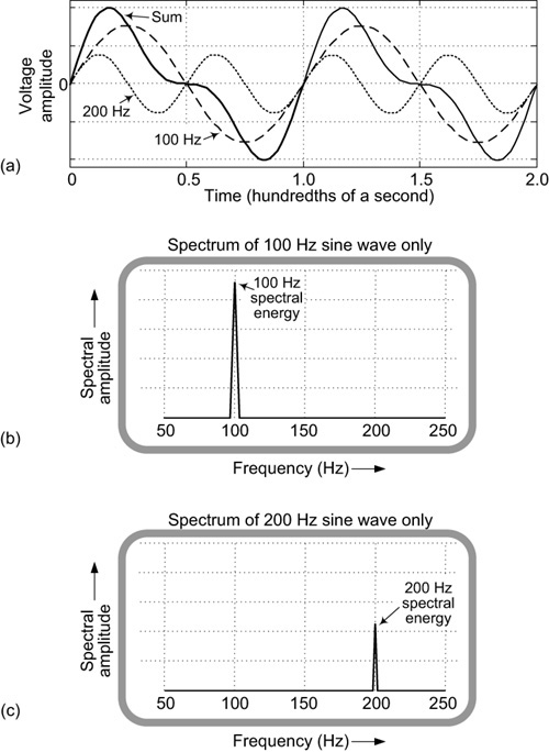
Figure 3-7 A 100 Hz sine wave and a 200 Hz sine wave: (a) time waveforms; (b) spectrum of the 100 Hz wave; (c) spectrum of the 200 Hz wave.
The spectra of the 100 Hz and 200 Hz sine waves are shown in Figures 3-7(b) and 3-7(c), respectively. Because the amplitude of the 100 Hz wave is greater than the amplitude of the 200 Hz wave in Figure 3-7(a), the height of the spectral energy spike of the Figure 3-7(b) is greater than the height of the spectral energy spike in Figure 3-7(c).
If we added the 100 Hz sine wave and the 200 Hz sine wave, the result would be the composite Sum waveform shown as the solid-line curve in Figure 3-7(a). Notice that at any instant in time the solid-line Sum waveform is the sum of the dashed-line and dotted-line waves at that instant in time. For example, at the time instant of 1.25 hundredths of a second, the dotted 200 Hz curve equals zero, so the Sum curve is equal to the 100 Hz curve. At that instant in time, the Sum wave equals the 100 Hz wave plus zero.
The spectrum of the composite Sum wave in Figure 1-17(a) is shown in Figure 3-8. The spectrum in Figure 3-8 is the sum of the Figure 3-7(b) and Figure 3-7(c) spectra. From Figure 3-8 we learn one of the most important properties of analog signals:
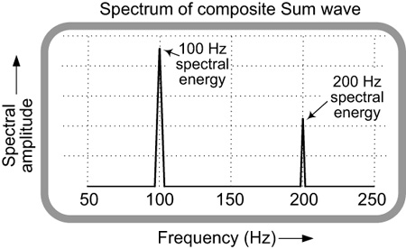
The spectrum of the sum of two analog time waves is equal to the sum of the waves’ individual spectra.
Harmonics
There’s an important topic we now introduce with regard to the spectrum of analog signals. That topic is harmonics, the undesirable spectral components in a time signal that cause an inadvertent distortion of the shape of the time signal. We start our discussion of harmonics by referring to the time-domain curves in Figure 3-9(a). In that figure, we see a high-amplitude 2 Hz sine wave represented by the solid-line curve. The figure also shows lower-amplitude 6 Hz and 10 Hz sine waves represented by the dashed- and dotted-line curves, respectively.
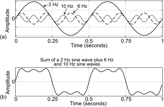
Figure 3-9 A 2 Hz analog square wave signal: (a) fundamental 2 Hz sine wave and its first two odd harmonics; (b) fundamental sine wave plus its first two odd harmonics.
If we add those three Figure 3-9(a) sinusoids together the sum is the waveform shown in Figure 3-9(b). If you’ll forgive the corny analogy, we can say that if you add 1/4 cup of a 2 Hz sine wave, plus 4 teaspoons of a 6 Hz sine wave, plus 2.5 teaspoons of a 10 Hz sine wave, the combination would be the waveform in Figure 3-9(b). There, we see the Sum waveform looks much like a square wave. The 6 Hz and 10 Hz sine waves are called the “odd harmonics of the 2 Hz sine wave.” That’s because 6 and 10 are integer multiples of 2; that is, 6 = 3 × 2 and 10 = 5 × 2. The numbers 3 and 5, both of which are odd numbers, are integers (whole numbers). We’re free to call the Figure 3-9(b) waveform a “2 Hz square wave” because it repeats itself twice in the time interval of one second.
In addition, adding the low-amplitude levels of 14 Hz (7 × 2) and 18 Hz (9 × 2) harmonic sine waves, shown in Figure 3-10(a), to the sum of sine waves in Figure 3-9(b) results in the even more square-like square wave we see in Figure 3-10(b).
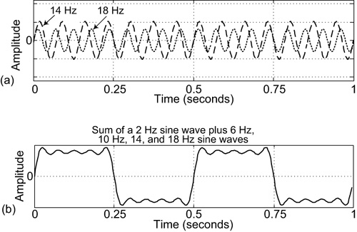
Figure 3-10 A 2 Hz square wave signal: (a) fundamental 14 Hz and 18 Hz sine waves; (b) fundamental 2 Hz sine wave plus its first four odd harmonics.
You can see what’s happening here. The more of its odd harmonics we add to a 2 Hz sine wave, the closer the summation waveform looks like a 2 Hz square wave. And that’s why we can say that a square wave is made up of, or comprises, a fundamental frequency sine wave plus that sine wave’s odd harmonics. There’s nothing sacred about starting with a 2 Hz sine wave here. We could just as well add a 5 kHz (5,000 Hz) sine wave to its odd harmonic sine waves of 15 kHz, 25 kHz, 35 kHz, and 45 kHz and obtain the square waveform in Figure 3-10(b) that repeats itself 5,000 times in one second.
The spectrum of the Figure 3-10(b) waveform is shown in Figure 3-11. The 2 Hz spectral component in Figure 3-10 is called the “fundamental frequency” because the Figure 3-10(b) waveform’s repetition rate is two repetitions per second (two cycles/second).
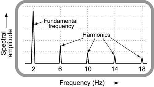
Your authors realize that spectral plots like Figure 3-11 may be new and a bit puzzling to many readers. Signal processing engineers interpret that figure as follows: Figure 3-11 simply tells us that a time waveform, shown in Figure 3-10(b), contains some given amplitude of a 2 Hz sine wave, plus a lower amplitude 6 Hz sine wave, plus lower-amplitude 10 Hz, 14 Hz, and 18 Hz sine waves.
To illustrate that a square wave really does contain odd harmonics, let’s say we built an audio detection system, containing a microphone carefully designed to detect the presence of an 18 Hz sine wave audio tone. When an 18 Hz audio tone is detected, the system turns on a red warning light. Now, if we connected the 2 Hz square wave voltage shown in Figure 3-10(b) to the terminals of a loudspeaker, the 18 Hz detection system’s warning light would suddenly light up. The audio tone detection system would identify the 2 Hz audio square wave’s 18 Hz harmonic component that we showed in Figure 3-11. Single-frequency sine wave voltages contain no harmonics but square wave voltages certainly do.
One consequence of this harmonics discussion is that we learn one of the most important principles in all of signal processing. That is:
A time signal having very abrupt (sudden) amplitude changes, like a square wave, contains higher-frequency spectral content than a single-frequency sinusoidal signal that has more gradual (smooth) amplitude changes.
This characteristic must be anticipated during the design of all analog and digital signal processing systems.
Harmonic Distortion
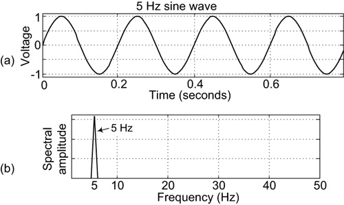
In practice, harmonics can be detrimental. Here’s why: think of the nice clean analog 5 Hz sine wave shown in Figure 3-12(a) with its frequency-domain spectrum that is shown in Figure 3-12(b).
Now let’s say the 5 Hz sine wave voltage in Figure 3-12(a) was applied to an amplifier whose operation was flawed, and the output of the amplifier is the distorted voltage waveform shown in Figure 3-13(a). The amplifier’s imperfect performance flattened the positive and negative peaks of the original pure sine wave input signal. That distortion is called harmonic distortion because the spectrum of the amplifier’s output signal contains unwanted harmonic spectral components as depicted in Figure 3-13(b). Let’s be clear now: The harmonics in Figure 3-13(b) did not cause the distorted waveform in Figure 3-13(a). The fact that the Figure 3-13(a) waveform is distorted is what produced the harmonics in Figure 3-13(b).
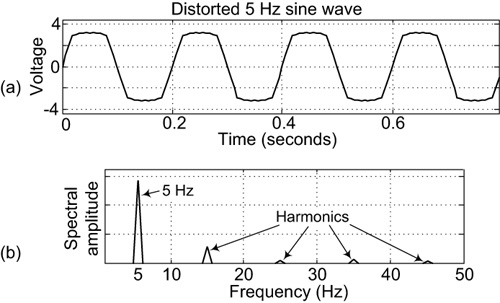
Figure 3-13 A distorted 5 Hz sine wave voltage: (a) time-domain plot; (b) frequency-domain spectrum showing harmonic distortion.
As an engineering example of harmonic distortion, if we replaced the analog sine wave in Figure 3-12(a) with the radio signal produced by a broadcast radio station, the distorted output of an imperfect amplifier would be the desired radio station signal plus copies of that signal centered at higher frequencies. That scenario is strictly forbidden. We don’t want harmonics from one radio station interfering with the signal from another station in a nearby city. That’s why the transmitters of broadcast radio stations are carefully designed to radiate signals only at their Federal Communications Commission–specified frequencies. Likewise, your cell phone contains carefully designed filters so that it does not radiate undesirable, high-frequency, harmonic electromagnetic energy. We don’t want your phone’s transmitted signal to interfere with someone else’s phone transmissions.
However, with audio signals, harmonics can be a good thing. Musical instruments generate an audio tone plus distinctive multiple audio harmonics. These harmonics allow us to tell musical instruments apart. Without harmonics, a piano playing a middle-C note would sound the same as a guitar playing middle C.
Decades ago, rock-n-roll guitarists realized that if they applied unusually high-level electric guitar signals to their vacuum-tube amplifiers, shortcomings in those amplifiers would produce musical notes suffering from high harmonic distortion such as that in Figure 3-13(b). The result was musical notes super-rich in roaring harmonic content, a sound that the rock guitarists liked. When transistor amplifiers came along, with their improved performance, the harmonic distortion was reduced so some rock guitarists weren’t happy with the first transistor amplifiers. This made the old vacuum-tube amplifiers highly sought after. Rumor has it that Rolling Stones lead guitarist Keith Richards still prefers vacuum-tube amplifiers. Because Richards has not returned our phone calls, your authors cannot confirm this rumor.
Bandwidth
Now that we’ve covered the basics of analog signal spectra, we can proceed to another important topic, signal bandwidth, which is the frequency range over which a signal contains significant spectral energy. A good way to start our bandwidth discussion is by considering old landline telephone systems.
The audio spectrum of human speech looks something like the curve shown in Figure 3-14(a). When people speak into the microphone of a landline telephone, their speech signals contain spectral energy that covers a frequency range of roughly 80 Hz to 7 kHz (7,000 Hz), so it’s reasonable to say that human speech has a bandwidth of 7 kHz.
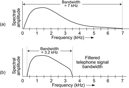
Figure 3-14 Human speech bandwidth: (a) full spectral bandwidth; (b) spectral bandwidth after telephone company filtering.
For a number of practical engineering reasons, the telephone company requires that an analog telephone speech signal contain energy only over a frequency range of somewhat less than 4 kHz. As a result, at the telephone company’s facility a telephone speech signal is passed through an analog filter that effectively eliminates spectral energy below 300 Hz and above about 3.5 kHz. Thus, the audio signal that the telephone company transmits from one telephone to another is limited in its bandwidth to 3.2 kHz, as shown in Figure 3-14(b).
There are a number of different definitions for bandwidth used by engineers. However, for now we’ll consider the word bandwidth to mean the frequency range over which a signal contains significant spectral energy. The reason the telephone company could limit the bandwidth of analog speech signals to 3.2 kHz is because most of the spectral energy of human speech is in the range of 300 Hz to 3.5 kHz, and humans can easily understand a speech signal that is limited in bandwidth to 3.2 kHz. It’s not high-fidelity speech, but certainly good enough to hold a conversation over the telephone.
Amplitude modulation (AM) radio stations broadcast audio signals that have bandwidths of 5 kHz. That’s why the audio from your AM radio sounds better than telephone audio. Better still, frequency modulation (FM) radio stations broadcast audio signals, for each of the left and the right channels, that have bandwidths just slightly less than 15 kHz. That’s why orchestra music sounds so good coming from an FM radio station. Audio geeks refer to FM audio as high fidelity. (Appendix C provides additional information concerning AM and FM radio signals.)
Let’s conclude our analog-signal bandwidth discussion by returning to an audio signal we discussed earlier. Figure 3-15(a) shows the spectrum of Capt. Kirk’s “Mister Spock” audio speech signal in Figure 2-12(a). Note that Figure 2-12(a) is a time-domain plot and Figure 2-15(a) is a frequency-domain plot. In Figure 3-15(a), we see that the speech signal has a bandwidth of roughly 4 kHz.
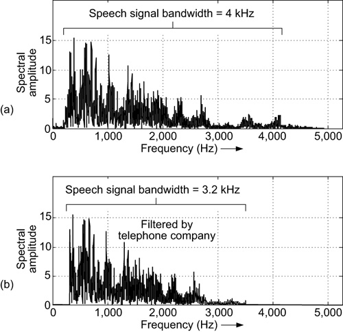
If that audio speech voltage signal had been passed through the telephone company’s filter, which only passes spectral energy in the range of 300 Hz to 3,500 Hz, the output spectrum of the filter would be that shown in Figure 3-15(b). Do you see the difference between the spectra in Figure 3-15(a) and Figure 3-15(b)? There you go—you now have experience in examining signal spectra! Because the vast majority of the spectral energy in Figure 3-15(a) does pass through the filter, the filtered speech signal would be easily perceptible at the receiving telephone’s loudspeaker output.
The Other Bandwidth
Unfortunately, there is an incorrect definition of the word bandwidth that’s very common nowadays. When you buy a new cell phone, the salesperson may tell you something like, “Your phone’s bandwidth is 1.4 megabits/second.” What he or she should have said was, “Your phone’s binary data transfer rate is 1.4 megabits/second.” (We explain binary bits in a later chapter.) For us, the term bandwidth has the very specific meaning of the width of a frequency band, measured in Hz, not a binary data transfer rate.
We don’t know just when the word bandwidth began to be used to describe binary data transfer rates but, sadly, that misnomer is surely here to stay.
What You Should Remember
In this chapter, we covered the concept of frequency as well as how we can describe an analog signal by its frequency-domain spectrum. All of the concepts we learned about the spectra of analog signals will help us understand digital signals.
The concepts you should remember from this chapter are:
• Periodically varying voltages, like sine and cosine wave voltages, are common in the world of signal processing.
• The repetition rate, per unit time, of a periodic voltage is called frequency.
• Frequency is most commonly measured in units of hertz (Hz). One Hz is equal to one cycle per second.
• We can describe analog signals by their frequency-domain spectral content.
• The spectrum of periodically varying voltages, except single-frequency sine and cosine wave voltages, contains a fundamental frequency component plus harmonic frequency components (higher frequency sinusoids).
• The frequency range over which a signal contains significant spectral energy is called the bandwidth of the signal.