5. Sampling and the Spectra of Digital Signals
This chapter explains what digital signal processing engineers mean when they talk about the topics of sampling and the spectra of digital signals. Both subjects are important as well as interesting and, after reading this chapter, you’ll understand the meaning of this terminology.
In Chapter 2, we introduced the idea of analog signals. These are signals whose voltage amplitudes smoothly change in value as time passes. Then in Chapter 3, we discussed the important notion of the spectrum of an analog signal, which is a description, or measure, of the frequency content of an analog signal. Although you’re usually not concerned with the spectra of analog signals in your daily life (unless you’re tuning a guitar or a piano), spectrum analysis is of profound and fundamental importance to signal processing engineers. In Chapter 4, we described the idea of a digital signal, a sequence of numbers faithfully representing an analog signal. In this chapter, we examine the concept of the spectra of digital signals. Familiarity with these spectra is essential for anyone wanting to understand the fundamentals of digital signal processing.
And as it turns out, with respect to spectral content, surprising things happen when we convert an analog signal to its digital signal representation. This chapter explains the important characteristics of such digital spectra. With that said, let’s briefly review the key aspects of analog signal spectra in preparation for a solid understanding of digital signal spectra.
Analog Signal Spectra—A Quick Review
In Chapter 2, we looked at analog signals whose voltage waveforms vary in amplitude as time passes. For example, let’s say an analog engineer’s job is to design an electronic circuit that generates a 1,000 Hz sine wave audio tone for use as a beeper for a microwave oven. The engineer solders the appropriate electronic components to a printed circuit board in order to generate a sine wave, shown in Figure 5-1, whose voltage value smoothly fluctuates 1,000 times per second. If the engineer used speaker wire to connect that sine wave voltage to a loudspeaker, he’d hear a pure audio tone.
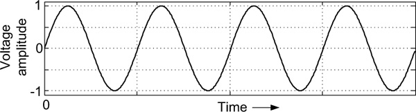
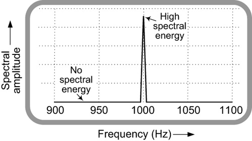
At that point, the audio tone generation task is only half finished. The engineer must next ensure that the spectrum, the frequency content, of his signal is indeed 1,000 Hz. (If it were 25,000 Hz, only his dog would hear it.) So the engineer applies the sine wave voltage to the input of a spectrum analyzer to display the spectrum of the audio signal. If the spectral display is that shown in Figure 5-2, the sine wave has the correct frequency spectrum and the engineer’s job is finished. The point of this little story is that not only is the time waveform shape of the audio signal important, but the spectrum of the signal is equally critical.
Another example of the importance of signal spectra involves commercial AM (amplitude modulation) radio broadcast stations. In the United States, AM radio broadcast systems are carefully designed so that their transmitted signals never have a spectral bandwidth greater than 10 kHz (10,000 Hz). In addition, the radio stations’ center frequencies (also called carrier frequencies) are carefully controlled so that they are separated by at least 10 kHz.
Figure 5-3 represents a hypothetical portion of the AM broadcast band. Radio Station #4’s center frequency is 640 kHz, separated by 10 kHz from the center frequencies of its neighboring stations as shown in Figure 5-3. To listen to Radio Station #4, we would tune our AM radio to a frequency of 640 kHz (or as the radio announcer would say, “Welcome to 640 on your radio dial”).
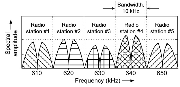
In Chapter 2, we stated that the bandwidth of AM radio audio signals is restricted to 5 kHz. That’s true; however, the inherent behavior of the amplitude modulation (AM) process, necessary so that signals can be transmitted using transmission antennas, doubles that audio signal’s bandwidth such that the radiated (broadcasted) signal has a bandwidth of 10 kHz as we see in Figure 5-3.
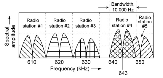
That 5 kHz audio bandwidth restriction is critical because if an equipment malfunction occurred at Radio Station #4 and the audio bandwidth was inadvertently 8 kHz, the radiated signal’s bandwidth would be 16 kHz as shown in Figure 5-4. That situation would cause Radio Station #4’s radiated signal to interfere with neighboring radio stations. The result would be that if you tuned your AM radio to Radio Station #3 or Radio Station #5, you’d hear some of the high-frequency audio from Radio Station #4 in the background of your desired station’s audio signal. Radio station engineers ensure this scenario never occurs.
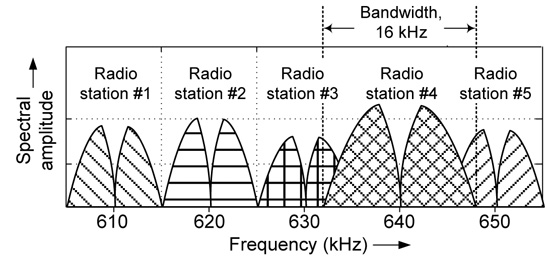
Figure 5-4 AM radio interference when Radio Station #4’s transmitted signal bandwidth exceeds 10 kHz.
The allocation of radio transmission center frequency and bandwidth has been a hot topic for many years. In the United States, the Federal Communication Commission (FCC) uses hearings, auctions, and even lotteries to allocate this finite and valuable resource. This is a far cry from the early days of communications in the 1800s when Morse code signals were sent using a spark-gap transmitter that radiated over very wide and unpredictable frequencies.
The restriction that an AM radio station’s transmitted signal center frequencies must be separated by exactly 10 kHz is also critical. Let’s say a transmitter equipment malfunction occurred at Radio Station #4 and its radiated signal’s center frequency was inadvertently 643 kHz as shown in Figure 5-5. That situation would cause Radio Station #4’s radio signal to interfere with Radio Station #5. To prevent one radio station’s signal from encroaching on another station’s signal, AM radio station engineers are tasked to see that the scenarios in Figure 5-4 and Figure 5-5 never occur. (Appendix C provides additional information concerning AM radio signals.)
The purpose of the discussion above is to show why we care so much about signal spectra. We cannot overemphasize the importance of controlling and measuring signal spectra in the practical world of signal processing. Having said that, let’s now look at the spectra of digital signals.
How Sampling Affects the Spectra of Digital Signals
When we convert an analog signal to a digital signal, the spectrum of the digital signal depends on two things: (1) the spectrum of the analog signal and (2) the fs sample rate of the analog-to-digital conversion process. This section explains that two-fold dependence.
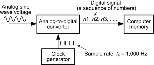
The vast majority of digital signals are generated by the periodic sampling process that we introduced in the last chapter. That process is shown in in Figure 5-6. We’ve seen the diagram in that figure before. An analog signal is applied to an analog-to-digital converter, whose sample rate is fs samples per second (commonly referred to as fs Hz), producing our digital signal, a sequence of discrete numbers.
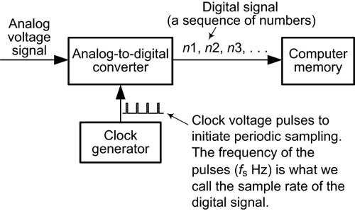
Figure 5-6 Generating a digital signal (the sequence of numbers n1, n2, n3, . . .) by sampling an analog signal.
Our goal in this sampling process is to generate a digital signal that includes all of the information contained in the input analog signal. For example, if the analog input signal is a music signal, we may want to assemble the digital signal’s samples (numbers) into a data file and attach that file to an e-mail and send it to a friend. Using the appropriate software on her home computer, our friend can use the digital signal data file to reproduce the original analog music signal and listen to it on her computer’s loudspeakers.
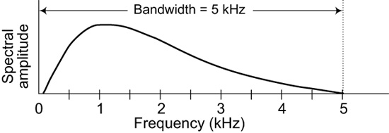
Thinking again about the notion of spectra, the analog voltage signal at the input of our sampling process will have some fixed spectrum. For example, if the analog signal is the output of a microphone, the signal may have a spectrum like that depicted in Figure 5-7.
The surprising thing about the periodic sampling process in Figure 5-6 is that the spectrum of the digital signal’s sequence of numbers not only depends on the spectrum of the analog input signal, but the spectrum of the digital signal also depends on the frequency of the fs sample rate! At first glance, that dependence may not seem too important, but indeed it is. If the analog input signal in Figure 5-6 has the spectrum shown in Figure 5-7, then we want the digital signal to have that same spectrum. In that case, the digital signal contains all the information, undistorted, that existed in the analog signal. However, it’s possible that, with an incorrectly chosen fs frequency for our clock pulses in Figure 5-6, the digital signal’s spectrum will not be the same as the analog signal’s spectrum. When that happens, the digital signal is a corrupted version of the input analog signal.
What we’re saying here is that with an improper fs sample rate, an analog music signal converted to a digital signal and e-mailed to a friend would sound like unintelligible audio garble on the friend’s computer loudspeakers. So, following that warning with regard to poorly chosen fs sample rates, let’s now take a closer look at what situations can cause unexpected, and possibly detrimental, digital signal spectral problems.
The Mischief in Sampling Oscillating Quantities
Before we examine the spectral effects of sampling analog signals, we’ll engage in another thought experiment.
Suppose we have a mechanical clock that has a second hand but no minute or hour hand. The second hand makes a full 360 degree rotation every 60 seconds. Next, suppose we take a photograph of the clock when the second hand is pointed at 12:00 noon and then take additional photos every 55 seconds. Our first four photographs would look like those in Figure 5-8(a) through Figure 5-8(d). We can think of those photographs as samples of the smooth, continuous rotary motion of the clock’s second hand.
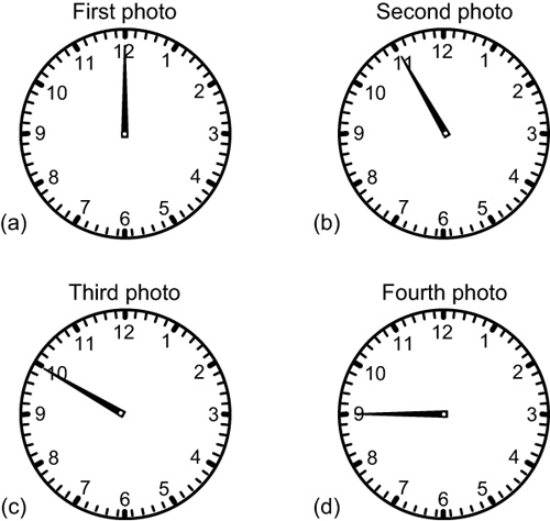
Upon showing those time-ordered photos in Figure 5-8 to someone, what would he or she think about the direction of motion of the second hand as time advances? That’s right; from the photos, it appears that the second hand is rotating in the counterclockwise direction! Now, if we took our photographs much more often, say once every 5 seconds, the time-ordered photos would look like those in Figure 5-9(a) through Figure 5-9(d). And in that figure, the sequence of photos correctly shows that the second hand is rotating in the clockwise direction.
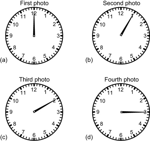
What we learn from our thought experiment is that sampling the clock’s continuously rotating second hand too slowly (one photo every 55 seconds) yields misleading results. Likewise, sampling the rotating second hand sufficiently often (one photo every 5 seconds) produces correct results. Further experimentation with photographs of our clock’s second hand shows us that the words sufficiently often mean that if we take photos more often than every 30 seconds, the sequence of photos would show the correct clockwise motion of the second hand. (If we took the photos exactly at 30-second intervals, the hand would alternate between the top and bottom of the clock, and we could not tell its direction of rotation.)
So, from this simple thought experiment we can state one of the most important principles in all of digital signal processing. That is:
To correctly represent a continuous (analog) periodic phenomenon whose cyclic period duration is t seconds with a sequence of samples, the time between samples must be less than half of t. For our clock, t is 60 seconds, so we must sample at intervals of less than 30 seconds.
Stated differently:
To correctly represent a continuous (analog) periodic phenomenon whose frequency is f cycles per second with a sequence of samples, the fs sample rate must be greater than two times f.
That last statement may not seem terribly profound, but it most certainly is. This sample rate restriction pervades essentially every aspect of digital signal processing.
You’ve seen that counterclockwise rotation illusion in Figure 5-8 before. In the old Western movies, recall that a wagon’s wheels sometimes appeared to rotate backward. That illusion occurred because the movie camera was taking a sequence of snapshots—a new snapshot 24 times per second. The spokes of a rotating wheel behave exactly like the clock’s second hand in our Figure 5-8 presentation. Depending on the rotation rate of the wagon wheel (in revolutions per second), its spokes may have appeared to be spinning far too slowly compared to the forward speed of the wagon. And in some case, the spokes even appeared to be rotating backward, the effect we saw in Figure 5-8.
Your cell phone’s video camera takes 20 to 30 pictures per second. You might try recording a cell phone video of a spinning electric fan, and turn the fan off while recording your video. Upon viewing your finished video, for a few moments the fan blades will appear to spin backward.
Next, we relate the sample rate restriction discussed above to the process of sampling an analog sine wave voltage in our quest to understand the spectra of digital signals.
Sampling Analog Sine Wave Voltages
In the last section, we introduced the notion that to correctly represent the behavior of a smoothly changing quantity (the position of a clock’s second hand) with samples, we must capture those samples (take photos of the second hand) at a sufficiently high sample rate. Let’s now relate that idea to sampling a simple analog sine wave voltage signal. Once we understand the behavior of sampling a sine wave signal, we’ll be able to understand more complicated examples of sampling, like the sampling of an audio signal on a music compact disc (CD).
Correct Sampling of an Analog Sine Wave
The process of sampling an analog sine wave voltage signal is depicted in Figure 5-10. An analog sine wave voltage is connected, by way of a two-wire cable, to the input of the analog-to-digital converter hardware. The output of the converter is a digital signal (a sequence of numbers) that is routed, by way of a multiwire cable, to a computer’s memory. Because the sample rate of this process is 1,000 Hz, 1,000 numbers per second are transferred to the computer. Using computer software, we can examine and display the values of our digital signal’s samples.
When the input analog sine wave voltage’s frequency is 200 Hz, the analog sine wave is shown by the solid curve in Figure 5-11(a) and the dots represent the discrete numbers produced by the analog-to-digital converter and stored in the computer’s memory.
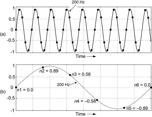
Figure 5-11 Sampling an analog sine wave voltage signal when the fs sample rate is 1,000 Hz: (a) sampling a 200 Hz sine wave; (b) the first six sample values.
If we zoom in on the first six samples of our digital signal, we see those sample values in Figure 5-11(b). For reference purposes, we include the dotted sine wave curve in Figure 5-11(b). There’s really nothing new here. This is merely the process of sampling an analog sine wave voltage, a process we first learned about in the last chapter.
We have correctly sampled Figure 5-11’s analog sine wave because our 1,000 Hz sample rate was greater than two times the frequency of the 200 Hz sine wave. We generated more than two discrete samples for each complete cycle of the analog sine wave. To be thorough, we list the first six samples of our digital signal in Table 5.1.
Incorrect Sampling of an Analog Sine Wave
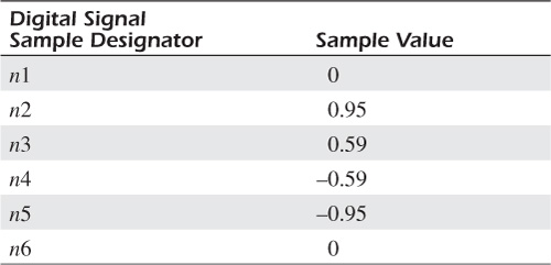
Let’s experiment a little: If we change the frequency of our input analog sine wave voltage from 200 Hz to 800 Hz, the first six samples of our digital signal would be the dots shown in Figure 5-12(a). And, if we change the frequency of the input analog sine wave from 800 Hz to 1,200 Hz, the first six samples of our digital signal would be the dots shown in Figure 5-12(b). Next, look very carefully at Figures 5-11(b), 5-12(a), and 5-12(b). Do you see anything interesting?
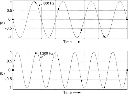
Figure 5-12 Sampling sine wave signals of different frequencies: (a) sampling an 800 Hz sine wave; (b) sampling a 1,200 Hz sine wave.
That’s right; the three digital signals (the three sets of dots) in those figures are identical! We verify this astounding situation by plotting the 200 Hz, 800 Hz, and 1,200 Hz sine waves and their digital representations in the rather busy Figure 5-13. From the discrete sample values alone, we cannot determine the original sine wave’s frequency. This situation is arguably the most astonishing consequence of dealing with sampled data.
The situation where a digital signal obtained from sampling a high-frequency analog sine wave takes on the identity of a digital low-frequency sine wave is called aliasing. Just as criminals may take on a new identity and a new name (an alias) to appear to be someone they are not, the 800 and 1,200 Hz digital sine wave signals appear identical to the sampled 200 Hz digital signal. This happens because we have not correctly sampled the 800 and 1,200 Hz analog sine waves. We did not generate more than two discrete samples for each complete cycle of those higher-frequency analog sine waves.
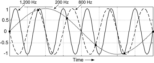
Figure 5-14 shows the incorrect sampling of the 800 and 1,200 analog sine waves. In the figure, the bold curves show complete cycles of the two analog sine waves where only one discrete sample is generated during those individual cycles.
Figure 5-14 Incorrect sampling showing where a complete analog cycle is represented by less than two samples: (a) an 800 Hz sine wave; (b) a 1,200 Hz sine wave.
Again, the point here is: from our digital signal alone (the sample values listed in Table 5.1), we cannot tell if that digital signal was obtained from sampling a 200, 800, or 1,200 Hz analog sine wave.
Why We Care about Aliasing
The situation where a digital signal can be the sampled representation of multiple sine waves having different frequencies, what we call aliasing, is of critical importance in the field of digital signal processing. We can easily demonstrate this importance with an example.
Earlier in this chapter, we mentioned the notion of converting an analog music signal into a digital signal, assembling the digital signal’s numerical samples into a data file, and e-mailing that file to a friend. Using appropriate software and the built-in digital-to-analog converter on her home computer, the friend can convert the digital signal file to an analog music signal and listen to it on her computer’s loudspeaker.
However, doing this with the digital signal in Figure 5-13 can lead to problems as we show in Figure 5-15. If the e-mailed digital signal was a sampled 200 Hz audio tone (sampled at a rate of 1,000 Hz), our friend would hear a 200 Hz tone from her computer’s speakers as shown in Figure 5-15(a). Things are as they should be.
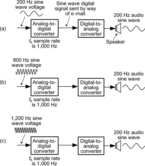
Figure 5-15 Reproducing an analog audio sine wave from a digital signal whose sample rate is 1,000 Hz: (a) original analog sine wave is 200 Hz; (b) original analog sine wave is the alias frequency 800 Hz; (c) original sine wave is the alias frequency 1,200 Hz.
On the other hand, if the original sampled analog signal were an 800 Hz audio sine wave as shown in Figure 5-15(b), our friend would still hear the reproduced analog sine wave as being a 200 Hz audio tone! Likewise, if the original sampled analog signal were a 1,200 Hz audio sine wave as shown in Figure 5-15(c), our friend would again hear the reproduced analog sine wave as being a 200 Hz audio tone. The scenarios in Figure 5-15 should not surprise us. That’s because the digital signals in all three e-mails are identical.
Now we know why 800 and 1,200 Hz sine waves are called aliases of a 200 Hz sine wave. After analog-to-digital conversion, both of these originally high-frequency sine waves will appear to be a low-frequency 200 Hz sine wave. That’s aliasing.
As it turns out, the highest frequency analog sine wave that we can correctly represent with digital samples is a sine wave whose frequency is no greater than half the sample rate. In our example above, the highest-frequency correctly sampled digital signal sine wave we can e-mail to our friend is a sine wave whose frequency is 1,000/2 = 500 Hz. So here we are, back to the topic we touched upon earlier in this chapter regarding taking photos of the rotating second hand of a clock. That is,
To correctly represent a continuous (analog) phenomenon whose highest frequency content is f cycles per second (Hz) with a sequence of samples, the fs sample rate must be greater than two times f.
In the field of digital signal processing, this sample rate restriction is called the Nyquist sampling criterion. This constraint is why modern telephone systems that transmit all phone calls as digital signals at a sample rate of fs = 8,000 Hz must filter all analog audio voice signals so that they contain no analog energy above 8,000/2 = 4,000 Hz, as we discussed in Chapter 3.
The Spectrum of a Digital Sine Wave Signal
Now we’re ready to answer the question, “What is the spectrum of a digital signal?” We answer that question with an example. Let’s say we sampled a 200 Hz analog sine wave at an fs sample rate of 1,000 Hz as shown in Figure 5-16(a). Figure 5-16(b) shows only the digital signal samples. Next, we compile the samples into a file and e-mail the file to a digital signal processing engineer. We tell the engineer that we sampled an analog sine wave and the digital signal’s sample rate is fs = 1,000 Hz. Being careful not to tell the engineer the original analog signal’s frequency, next we ask the engineer to determine the spectrum of the digital signal.
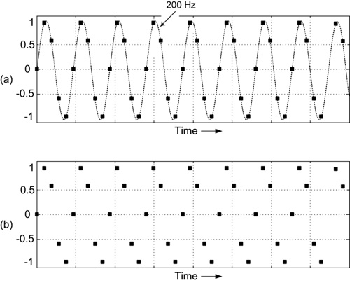
Figure 5-16 Sampling a 200 Hz sine wave at an fs sample rate of 1,000 Hz: (a) original analog sine wave (dashed curve) and digital signal samples; (b) digital signal samples only.
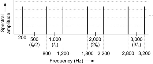
The engineer can perform a mathematical operation on the digital signal samples and determine that the signal has a frequency of one-fifth of the sample rate; that is 1,000/5 = 200 Hz. The engineer can then state that the sampled analog signal that produced the digital signal was a 200 Hz analog sine wave.
But, based on the concept of aliasing we presented in the last section, and an fs sample rate of 1,000 Hz, the engineer also knows that the original analog signal could also have been an 800, 1,200, 1,800, or 2,200, etc., Hz analog sine wave. Because of the inherent frequency-aliasing behavior of the process of sampling analog signals, the engineer is faced with a fundamental ambiguity of just what was the frequency of the original analog signal that was sampled to produce the digital signal.
Given this well-known frequency ambiguity, digital signal processing pioneers decided decades ago that the most realistic way to show the spectrum of the Figure 5-16(b) digital signal is the diagram in Figure 5-17. Given the digital signal sample values and the fs = 1,000 Hz sample rate, the engineer analyzing the digital signal has no choice but to create the Figure 5-17 graphical description, with its never-ending spectral replications. Now you understand why earlier in this chapter we wrote:
When we convert an analog signal to a digital signal, the spectrum of the digital signal depends on two things: (1) the spectrum of the analog signal and (2) the fs sample rate of the analog-to-digital conversion process.
However, let’s say we sent a second e-mail to the engineer stating, “By the way, we correctly sampled our analog sine wave. That is, the 1,000 Hz sample rate was greater than twice the frequency of the analog sine wave.” At that point, all frequency ambiguity is eliminated for the engineer. He now knows that the analog sine wave signal’s frequency was less than fs/2 = 500 Hz, and the only spectral component of the digital signal spectrum in Figure 5-17 that is less than 500 Hz is 200 Hz. Therefore, the sampled analog sine wave had a frequency of 200 Hz, allowing the engineer to graphically describe the spectrum of the digital signal as shown in Figure 5-18.
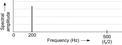
The point here is that the spectrum of the Figure 5-16(b) digital sine wave signal can be described by either Figure 5-17 or Figure 5-18. Both of these figures are correct, they contain the same amount of information, and, if given one of the figures, we could draw the other figure.
The Spectrum of a Digital Voice Signal
To enhance our understanding of the spectra of digital signals, let’s look at the spectrum of a digital signal that’s more complicated than a simple sine wave.
In Chapter 3, we presented an analog voice signal whose spectrum is that shown in Figure 5-19(a). If we apply that analog voice signal to an analog-to-digital converter, whose sample rate was fs = 8,000 Hz, the spectrum of the digital signal is shown in Figure 5-19(b).
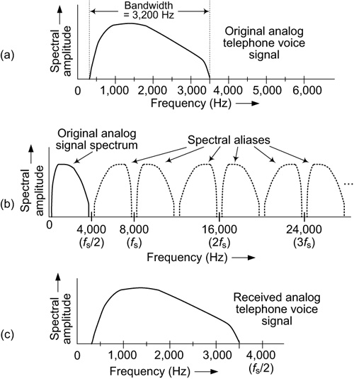
Figure 5-19 Telephone voice signal: (a) original analog signal spectrum; (b) digital signal spectrum showing spectral replications; (c) alternate depiction of the digital signal spectrum.
Because we know the fs = 8,000 sample rate is greater than twice the highest-frequency spectral component of the original analog voice signal, there is no frequency ambiguity (no overlapping spectral aliases) in Figure 5-19(b). Based on the spectrum of the digital signal, we know the spectrum of the original analog signal is that shown on the left side of Figure 5-19(b). As such, our digital signal’s spectrum can also be drawn, with equal validity, as that shown in Figure 5-19(c). Again, both Figure 5-19(b) and Figure 5-19(c) are correct and equivalent depictions of the digital signal’s spectrum.
The critical point about this topic of digital voice signals is the fact that the telephone company transmits the digital signal, whose spectrum is shown in Figure 5-19(b), from a switching station near the caller’s location to a switching station near the call recipient’s location. The switching station near the call recipient’s location converts that digital signal back to an analog signal whose spectrum is shown in Figure 5-19(c). The regenerated analog signal is then transmitted to the call recipient’s home telephone. Because the spectrum of the analog voice signal received by the call recipient is the same as the spectrum of the analog voice signal originally produced by the caller, as shown in Figure 5-19(a), the call recipient hears an intelligible voice from the loudspeaker of his landline telephone.
The Spectrum of a Digital Music Signal
Let’s consider audio music signals whose bandwidths are greater than the 3.2 kHz bandwidth of voice signals. Figure 5-20(a) shows the spectrum of a hypothetical analog music signal having a bandwidth of 6 kHz. The highest-frequency spectral content of the analog signal is roughly 6 kHz. If we used an analog-to-digital converter to sample that analog signal at a sample rate of fs = 8 kHz, the spectrum of the resulting digital signal would be that shown in Figure 5-20(b). Let’s assume we’ve recorded the digital signal on a compact disc (CD).
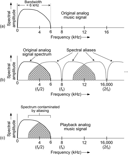
Figure 5-20 Hypothetical analog music signal: (a) original music signal spectrum; (b) digital signal spectrum showing overlapped spectral replications; (c) contaminated spectrum of the analog playback signal from a CD.
Because the fs = 8 kHz sample rate is less than twice the highest-frequency spectral content of the analog signal (that is, less than 12 kHz), a spectral alias overlaps the original signal spectrum as shown by the cross-hatched area on the left side of Figure 5-20(b). In this scenario, we have violated the Nyquist sampling criterion, which results in a digital signal whose low-frequency spectrum is contaminated. As such, if we put that compact disc in a CD player to listen to the music, the audio signal we hear will have the spectrum shown in Figure 5-20(c). The digital signal’s overlapped spectral components cause the final analog audio playback signal to have an unpleasant underwater, or gurgling, sound.
Audio engineers who record music on CDs solve the overlapped spectrum problem described above by merely increasing the fs sample rate of the digital signal obtained from the original analog music signal. Because analog music signals can have frequencies almost as high as 20 kHz, as shown in Figure 5-21(a), the sample rate of the digital music signals recorded on music CDs must be greater than 40 kHz. For a variety of engineering reasons, the industry standard sample rate for music compact discs is 44.1 kHz as shown in Figure 5-21(b). In that figure, we see that the fs = 44.1 kHz sample rate results in no spectral overlap and the CD’s analog playback signal will be undistorted as shown in Figure 5-21(c).
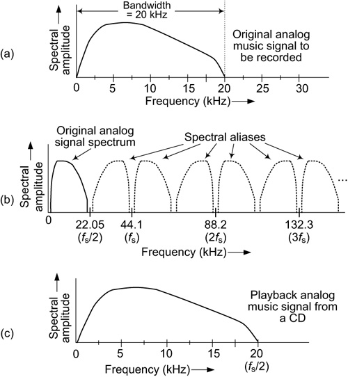
Figure 5-21 Analog music signal: (a) original music signal spectrum; (b) digital signal spectrum showing no overlapped spectral replications; (c) spectrum of the analog playback signal from a CD.
Anti-Aliasing Filters
In the field of digital signal processing, you’re likely to encounter the phrase anti-aliasing filter. Such a filter is a hardware device, and we describe its operation by way of a practical example.
Think about a large electric AC power transformer, such as that shown in Figure 5-22, sitting on concrete platform just outside the outer wall of a restaurant or hotel. If you’ve ever stood next to such a transformer, you may recall how it emits a low-frequency audio hum—a continuous insect-like buzzing. The fluctuating AC voltage inside the transformer generates a fluctuating magnetic field that causes metal plates within the transformer to vibrate. Just as the vibrating cone of a loudspeaker generates sound, the transformer’s internal metal plates vibrate and produce a low-level 120 Hz audio hum (or 100 Hz if you live in Europe). Commercial transformer manufacturers do their best to minimize their transformers’ audio humming noise. To do so, they must first measure the amplitude (the loudness) of that 120 Hz audio humming signal.

So let’s say it’s our job to measure the amplitude of the audio humming sound in close proximity to a large AC power transformer. Our test setup will be that shown in Figure 5-23(a). In measuring the amplitude of a 120 Hz audio signal, we must satisfy the Nyquist sampling criterion by setting the analog-to-digital converter’s fs sample rate to be greater than two times 120 Hz. So we’re free to choose a sample rate of fs = 300 Hz as shown in Figure 5-23(a).
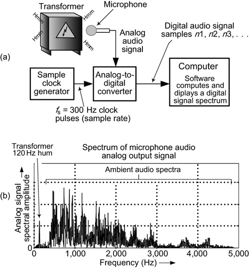
Figure 5-23 Measuring an AC power transformer’s humming 120 Hz audio signal: (a) test equipment setup; (b) spectrum of the microphone’s analog output signal.
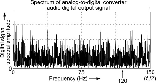
Let’s assume the spectrum of the microphone’s analog audio output signal is as shown in Figure 5-23(b). We see our low-level 120 Hz humming signal’s spectral component on the left side of the figure, as well as higher-frequency ambient audio spectral energy caused, for example, by nearby automobile traffic. Again, our job is to measure the amplitude of the 120 Hz signal’s spectral component.
Upon computing and displaying the spectrum of our analog-to-digital converter’s output signal, shown in Figure 5-24, we encounter a big problem: Due to the inherent behavior of sampling our analog signal, the microphone output signal’s high-frequency audio spectral energy aliases down in frequency to appear as the low-frequency spectral energy displayed in Figure 5-24. The 120 Hz spectral amplitude peak value we want to measure is severely contaminated, and essentially obscured, by aliased spectral energy.
The solution to our problem is to eliminate the high-frequency spectral energy in the analog signal applied to our analog-to-digital converter, and we do so with the analog lowpass anti-aliasing filter shown in Figure 5-25(a). That analog filter is built to pass low-frequency signals, including our desired 120 Hz signal, and drastically reduces all spectral energy above 120 Hz. Thus, the spectrum of the analog signal applied to the analog-to-digital converter is as shown Figure 5-25(b).
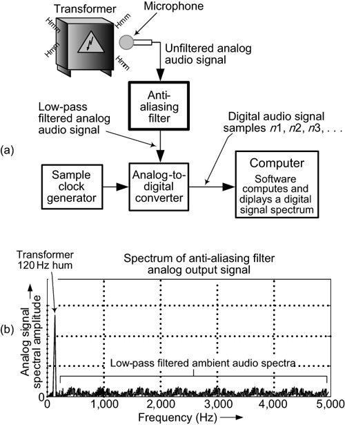
Figure 5-25 Using an anti-aliasing filter to measure a 120 Hz audio signal: (a) new test equipment setup; (b) spectrum of the filter’s analog output signal.
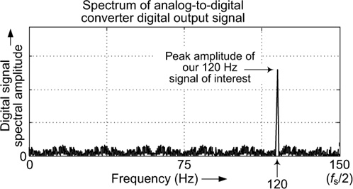
By employing an analog anti-aliasing filter, the ambient high-frequency spectral energy above 120 Hz in Figure 5-25(b), applied to the analog-to-digital converter, is very low in amplitude. So when that unwanted high-frequency, low-amplitude, energy aliases down in frequency in our digital signal’s spectrum, as shown in Figure 5-26, it does not inhibit our ability to measure the spectral peak amplitude of our desired 120 Hz signal. Using the hardware analog anti-aliasing filter is mandatory for success in this situation.
Analog-to-Digital Converter Output Numbers
An important topic regarding the process of sampling an analog signal is the nature of the numbers produced by an analog-to-digital converter.
When we sample an analog signal, as shown in Figure 5-25(a), the digital signal’s sequence of numbers is not in the form of the decimal numbers that we’re so familiar with in our daily lives. The digital signal’s sequence of numbers, n1, n2, n3, . . . , is in the form of what we call binary numbers. The interesting topics of binary numbers and why we use them are discussed in Chapter 9.
• To correctly represent a continuous (analog) phenomenon whose highest frequency content is f cycles per second (Hz) with a sequence of samples, the sample rate must be greater than two times f (the Nyquist sampling criterion).
• After analog-to-digital conversion using a sample rate of fs Hz, any sampled analog sine wave whose frequency is greater than fs/2 Hz will always be translated down in frequency to be in the range of zero Hz to fs2 Hz.
• Any digital sine wave signal (a sequence of discrete samples), such as that in Figure 5-13, represents a sampled version of an infinite number of high-frequency analog sine waves.
• In many real-world applications of sampling analog signals, hardware anti-aliasing filters are used to eliminate the unwanted high-frequency content of an analog signal applied to an analog-to-digital converter.