7. Wavelets
There is a discipline in the field of digital signal processing called wavelets. As we’ll explain here, wavelet transforms are similar to Fourier transforms except that with wavelets, we can find both the frequency and the time of interesting signal characteristics. Wavelet processing is used extensively in signal and image processing, medicine, finance, radar, sonar, geology, and many other varied fields. Wavelets are usually presented in mathematical formulae, but can actually be understood in terms of simple comparisons with the signal data we are analyzing.
To provide some background, we first look at the fast Fourier transform (FFT). That transform can be thought of as a series of comparisons with your data, which for now we will call a signal for consistency. Signals whose frequency content does not change over time can be processed with ordinary FFT methods.
Real-world signals, however, often have frequencies that change over time or have pulses, anomalies, or other events at certain specific times. This type of signal can tell us where something is located on the planet, the health of a human heart, the position and velocity of a blip on a radar screen, stock market behavior, or the location of underground oil deposits. For these signals, wavelet analysis has the capability to show not only the spectral content of a signal, but also to indicate when in time those spectral components exist. That is a very powerful signal analysis capability. We now demonstrate both the fast Fourier and wavelet transforms of a simple pulse signal.
The Fast Fourier Transform (FFT)—A Quick Review
We start with a point-by-point comparison of the pulse signal (D) with a high-frequency sinusoid wave of constant frequency (A) as shown in Figure 7-1. We obtain a single goodness value from this comparison (a correlation value), which indicates how much of that particular sinusoid wave is found in our pulse signal.
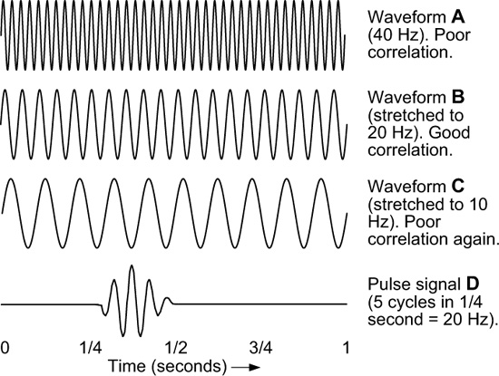
We can observe that the pulse D has 5 cycles in one-quarter of a second. This means it has a frequency of 20 cycles in one second or 20 Hz. The comparison sinusoid, A, has twice the frequency or 40 Hz. Even in the area where the D signal is non-zero (the pulse), the comparison is not very good.
By lowering the frequency of A from 40 to 20 Hz (waveform B), we are effectively stretching the sinusoid (A) by 2 so it has only 20 cycles in 1 second. We compare point-by-point again over the 1-second interval with the pulse D. This correlation gives us another value that indicates how much of this lower frequency sinusoid (now the same frequency as our pulse) is contained in our pulse signal. This time, the correlation of the pulse with the comparison 20 Hz sinusoid is very good. The peaks and valleys of B and the pulse portion of D align (or can be easily shifted to align) and thus we have a large correlation value.
Figure 7-1 shows us one more comparison of our original sinusoid A stretched by 4 so it has only 10 cycles in the 1-second interval, C. The comparison of the 10 Hz sine wave with pulse signal D is again poor. We could continue stretching until the comparison sine wave becomes a straight line having zero frequency, but all those comparisons will be increasingly poor.
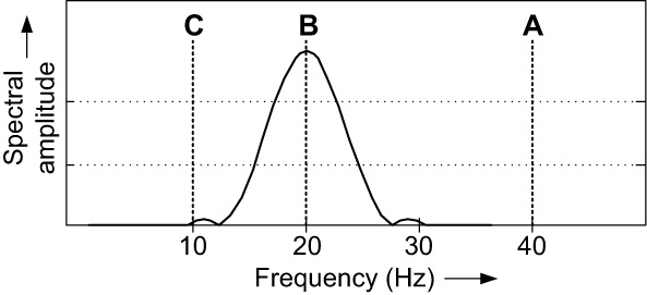
A fast Fourier transform (FFT) compares many stretched sinusoids to the pulse rather than just the 3 shown in Figure 7-1. The best correlation is found when the sinusoid frequency best matches the frequency of the pulse. Figure 7-2 shows the first part of an actual FFT of our pulse signal D. The locations of our sample comparison sinusoids A, B, and C are indicated. Notice that the FFT correctly tells us that the pulse has primarily a frequency of 20 Hz, but does not tell us where the pulse is located in time!
The Continuous Wavelet Transform (CWT)
Wavelets are exciting because they, too, are comparisons, but instead of correlating with various stretched, infinite-length, unchanging sinusoids, they use smaller or shorter waveforms (wave-lets) that can start and stop where we wish.
Using what is called the continuous wavelet transform (CWT), by stretching and shifting the wavelet numerous times we obtain numerous correlations. If our signal under analysis has some interesting events embedded in it, we will get the best correlation when the stretched wavelet is similar in frequency to the event and is shifted to line up in time with the event. Knowing the amounts of stretching and time shifting, which produce large comparison result values, we can determine both the frequency, and time of occurrence, of interesting events within a signal.
Figure 7-3 demonstrates the process. Instead of sinusoids for our comparisons, we will use wavelets. Waveform A shows what is called a Daubechies 20 wavelet about one-eighth of a second long that starts at the beginning (t = 0) and effectively ends well before one-quarter of second. The zero values are extended to the full 1 second. The point-by-point comparison with our pulse signal D will be very poor and we will obtain a very small correlation value.
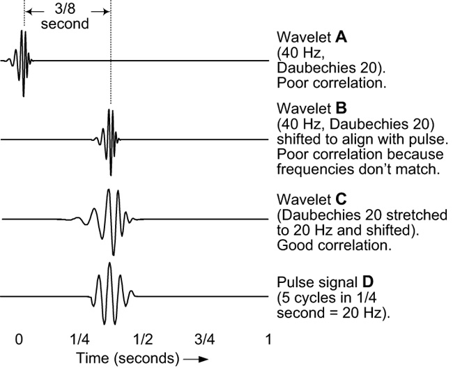
In the previous FFT discussion, we proceeded directly to stretching. In wavelet transforms, we shift the wavelet slightly to the right and perform another comparison with this new waveform to get another correlation value. We continue to shift until the Daubechies 20 wavelet is in the three-eighths-of-a-second time position shown in B. We get a little better comparison than A, but it’s still very poor because B and D are different frequencies.
After we have shifted the wavelet all the way to the end of the 1-second time interval, we start over with a slightly stretched wavelet at the beginning and repeatedly shift to the right to obtain another full set of these correlation values. C shows the Daubechies 20 wavelet stretched to where the frequency is roughly the same as the pulse (D) and shifted to the right until the peaks and valleys line up fairly well. At this particular shifting and stretching, we should obtain a very good comparison and large correlation value. Further shifting to the right, however, even at this same stretching, will yield increasingly poor correlations.
In the continuous wavelet transform (CWT), we have one correlation value for every shift of every stretched wavelet. To show the correlation (comparison) results of all these stretches and shifts, we use a three-dimensional display with the stretching (roughly the inverse of frequency) as the vertical axis, the shifting in time as the horizontal axis, and brightness to indicate the strength of the correlation. Figure 7-4 shows a continuous wavelet transform display for the Figure 7-3 pulse signal (D). Note the strong correlation (bright areas) of the peaks and valleys of the pulse with the Daubechies 20 wavelet, the strongest (brightest) being where all the peaks and valleys best align.
Figure 7-4 shows that the best correlation occurs at the brightest points, between one-quarter and one-half of a second. This agrees with what we already know about the pulse (D). Figure 7-4 also tells us how much the wavelet had to be stretched (or scaled) and this indicates the approximate frequency of the pulse in our pulse signal. Thus, we know not only the frequency of the pulse, but also the time of its occurrence!
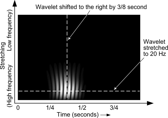
Figure 7-4 CWT display indicating the time and frequency of the pulse signal. (White bands show at what time the peaks and valleys of both the signal and the wavelet are aligned.)
We run into this simultaneous time/frequency concept in everyday life. For example, a bar of sheet music may tell the pianist to play a C chord of three different frequencies at exactly the same time on the first beat of the measure.
For the simple Figure 7-3 example, we could have just looked at the pulse (D) to see its location and frequency. The next example is more representative of wavelets in the real world.
Figure 7-5(a) shows a sine wave signal with a very small, very short-time discontinuity at Time = 180. The amplitude versus time plot of the signal does not show the tiny event. A standard fast Fourier transform (FFT) amplitude versus frequency plot would tell us what frequencies are present in the imperfect sine wave signal but would not indicate at what value of time those frequencies existed.
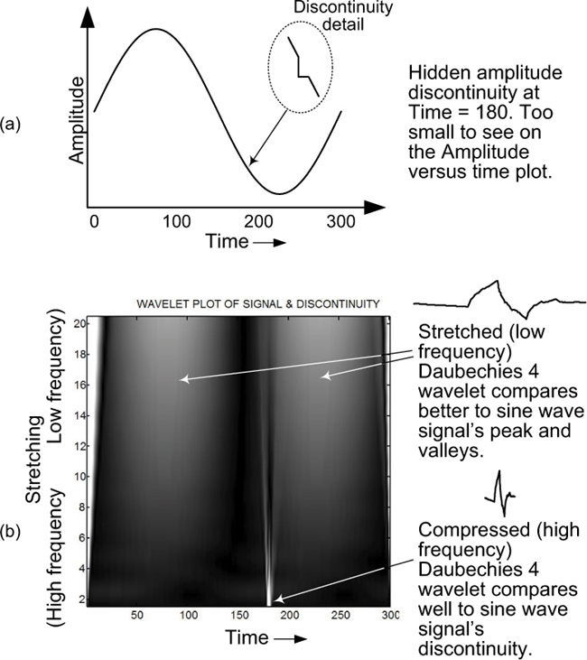
Figure 7-5 Detecting a small amplitude discontinuity: (a) sine wave signal containing a hidden discontinuity at Time = 180; (b) CWT of a sine wave signal with a hidden discontinuity.
With the wavelet display in Figure 7-5(b), however, at the bottom of that figure we can clearly see a vertical white band at Time = 180 at low scales when the wavelet has very little stretching, indicating a very high frequency. But more important to us, this tiny discontinuity has been precisely identified in time. The CWT display also finds the large oscillating wave at the higher scales where the wavelet has been stretched and compares well with the lower frequencies. For this short discontinuity, we used a short wavelet called a Daubechies 4 wavelet for best comparison.
This is an example of why wavelets have been referred to as a mathematical microscope for their ability to find interesting events of various lengths and frequencies hidden in signal data.
By the Way
The continuous wavelet transform as computed on a digital computer is, of course, not really continuous in the analog signal sense we have discussed in this book. In wavelet jargon, it means that we compute so many more discrete sequence samples (all the possible integer factors of shifting and stretching) than in the short-sequence discrete wavelet transforms we are about to discuss, that it seems continuous by comparison.
You will encounter some very creative jargon in wavelets because established words have been given new definitions. Other examples, besides continuous, meaning more numerous, include: decimation by 2 (having nothing to do with the deci-prefix); dilation, meaning to make either larger or smaller; translation, meaning shifting; scaling, meaning stretching; and family-friendly terms such as mother, father, and daughter wavelets! As Humpty Dumpty said in Through the Looking Glass, “When I use a word, it means just what I choose it to mean—neither more nor less.”
Besides acting as a microscope to find hidden events in our signal data, wavelets can also separate the data into various frequency components, as does the fast Fourier transform (FFT). The FFT is used extensively to remove unwanted noise that is prevalent throughout the entire signal such as unwanted 60 Hz audio hum. Unlike the FFT, however, the wavelet transform allows us to remove frequency components at specific times within the signal data. This allows us a powerful capability to throw out the bad and keep the good part of the data in that frequency range.
The wavelet transforms we’re about to discuss are called discrete wavelet transforms (DWT). They also have easily computed inverse discrete wavelet transforms (IDWT) that allow us to reconstruct the signal after we have identified and removed the unwanted noise or superfluous signal data in noise-removal or image-compression applications.
Undecimated or Redundant Discrete Wavelet Transforms (UDWT/RDWT)
One type of DWT is the redundant discrete wavelet transform (RDWT), often called the undecimated discrete wavelet transform (UDWT) for reasons we will soon see. With the RDWT, we first compare (correlate) the wavelet filter with itself. This produces a highpass half-band filter or superfilter. When we compare or correlate our signal with this superfilter, we extract the highest half of the frequencies. For a very simple denoising, we could just discard these high frequencies (for whatever time period we choose) and then reconstruct a denoised signal.
Multi-level RDWTs allow us to stretch the wavelet, similar to what we did in the CWT, except that it is done by factors of 2 (2 times as long, 4 times as long, etc.). This allows us stretched superfilters that can be half-band, quarter-band, eighth-band, and so forth.
Conventional (Decimated) Discrete Wavelet Transforms (DWT)
We stretched the wavelet in the CWT and the RDWT. In the conventional DWT, we shrink the signal instead and compare it to the unchanged wavelet. We do this by decimating by 2. Every other point in the signal is discarded. We have to deal with aliasing (not having enough samples left to represent the high-frequency components and thus producing a false signal). We must also be concerned with shift invariance. (Do we throw away the odd or the even values? It matters!)
If we are careful, we can deal with these concerns. One amazing capability of the filters in the conventional DWT is alias cancellation where the basic wavelet and three similar filters combine to allow us to reconstruct the original signal perfectly. The stringent requirements for the wavelets to be able to do this are part of why they often look so strange, as we shall see.
As with the RDWT, we can denoise our signal by discarding portions of the frequency spectrum obtained from a conventional DWT—as long as we are careful not to throw away vital parts of the alias cancellation capability. Correct and careful decimation also aids with compression of the signal.
There is a very common operation used in the field of signal processing called image compression, which refers to reducing the size, measured in bytes, of a graphics (picture) file without unacceptable degradation of the image quality. Reducing an image’s file size enables us to store more images in a given amount of hard-disk memory as well as minimizing the time required to download or send images over the Internet. Modern JPEG image compression uses wavelets to produce the results demonstrated in Figure 7-6. An original image is shown in Figure 7-6(a), and a biorthogonal 9/7 wavelet-compressed version of that image is given in Figure 7-6(b). The big deal is that the left image file requires 157 times the number of bytes as the wavelet-compressed image on the right! Can you see any difference between the two images?
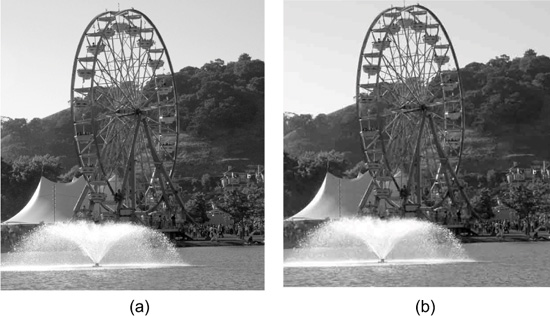
Figure 7-6 JPEG image compression using biorthogonal 9/7 wavelets: (a) before compression; (b) after compression.
By the Way
Thinking about JPEG image files, you may have also heard of MPEG video files. The file-name extensions “.jpg” and “.mpg” on your computer are their abbreviations. These are industry-standard electronic file compression methods. JPEG stands for Joint Photographic Experts Group and MPEG stands for Motion Picture Experts Group.
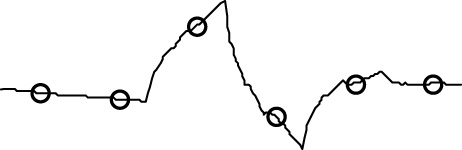
There are many types of wavelets. One type comes from mathematical equations while a second type is built from basic wavelet filters having as little as two points (two sample values). The Daubechies 4, Daubechies 20, and biorthogonal wavelets are examples of this second type. Figure 7-7 shows a 768-point approximation of a continuous Daubechies 4 wavelet with the four filter points (plus 2 zero-valued points) superimposed.
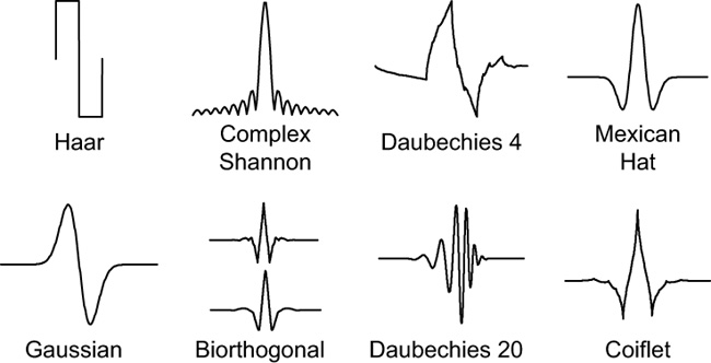
Some wavelets have symmetry (valuable in human vision perception) such as the biorthogonal wavelet pairs. Shannon or Sinc wavelets can find events with specific frequencies. Haar wavelets (the shortest) are good for edge detection and reconstructing binary pulses. Coiflet wavelets are good for signal data with self-similarities (fractals) such as financial trends. Some of the wavelet families are shown in Figure 7-8.
You can even create your own wavelets, if needed. However, there is an embarrassment of riches (too much of a good thing) in the many wavelets that are already out there and ready to use. We have already seen that, with their ability to stretch and shift, wavelets are extremely adaptable. You can usually get by very nicely with choosing a less-than-perfect wavelet. The only wrong choice is to avoid wavelets due to an overabundance of wavelet choices.
The time spent in learning and correctly using wavelets for the fascinating real-world signals that have anomalies, or sudden changes in frequency at specific times, will be handsomely repaid. More information on wavelets can be found at http://www.ConceptualWavelets.com.
What You Should Remember
The concepts you should remember from this chapter are:
• Wavelet transforms (wavelets) are mathematical processes allowing us to determine the spectrum of digital real-world signals having frequencies that change over time or have pulses, anomalies, or other events at certain specific times.
• Wavelets allow us to detect small amplitude discontinuities and other hidden events in digital signals.
• Wavelets are also used for image compression and are found in almost every modern digital camera and cell phone.
• There are many different types of wavelet transforms. They all stretch and shift and are very adaptable. However, one type may be better than another for a particular application (biorthogonal for images, Haar for short events, Daubechies 20 for chirp signals, Shannon for precise frequency determination, and so on).