
39
Measuring and Improving Pay for Performance: Board Oversight of Executive Pay
Stephen F. O'Byrne
President, Shareholder Value Advisors Inc.
Executive pay in public and private for-profit companies has three basic objectives: provide strong incentives to increase shareholder value, retain key talent, and limit the cost of executive pay to levels that will maximize the wealth of existing shareholders. The key responsibility of the board is to ensure that the company's executive pay program achieves the three basic objectives of executive pay.
In this chapter, I will argue that:
- The board cannot effectively discharge its responsibility without meaningful measures of incentive strength, that is, pay sensitivity to performance, and the pay premium at peer group average performance, what we call performance-adjusted cost.
- The measures commonly used for board oversight of executive pay—percent of pay at risk and competitive position—are very poor proxies for incentive strength and performance-adjusted cost.
- There is a simple, but very informative, analysis that provides measures of incentive strength and performance-adjusted cost that can be used for benchmarking and, more importantly, to understand the pay-plan design needed to achieve perfect pay for performance.
The chapter is organized in the following sections:
- The three basic objectives of executive pay.
- A brief history of executive pay.
- Why percent of pay at risk is not a meaningful measure of incentive strength.
- Measuring the three basic objectives of executive pay.
- The design implications of the measurement analysis: perfect pay plans.
- Benchmarking pay for performance.
- Executive pay has a big impact on shareholder wealth.
- Directors need to ensure that they themselves have strong incentives to increase shareholder value.
- Institutional investors don't do a good job on Say on Pay.
- ISS doesn't do a good job for institutional investors.
- Conclusion.
The Three Basic Objectives of Executive Pay
There is little disagreement that the key objectives of executive pay are providing strong incentives, retaining key talent, and limiting shareholder cost. Virtually every public company's proxy statement mentions performance incentives and retention as key compensation objectives. Limiting shareholder cost is rarely mentioned as an explicit objective, but is an implicit objective for every company. For example, Dow Chemical's four primary compensation objectives include “motivate and reward executives when they deliver desired business results and stockholder value” and “attract and retain the most talented executives to succeed in today's competitive marketplace.” Dow's other two objectives are just means of achieving strong shareholder incentives.1 Dow limits shareholder cost by targeting the median of its survey peer group, but its stated rationale for targeting the median is “to attract, motivate, develop, and retain top-level executive talent.”
A Brief History of Executive Pay
While the basic objectives of executive pay have never really changed, the common approach to executive pay is much different now than it was in the first half of the twentieth century. In the first half of the twentieth century, management incentive plans were largely value-sharing plans that provided strong incentives and controlled shareholder cost, but led to retention problems if a company did not build up an adequate bonus reserve in good times to maintain relatively competitive pay in bad times. The incentive plan adopted by General Motors in 1922 illustrates the common approach in the first half of the twentieth century. The plan made the total incentive pool equal to 10 percent of profit in excess of 7 percent of book capital. The pool covered all incentive compensation, both cash and stock, for all management employees at General Motors. The management share and threshold return were maintained without any change for 25 years. The plan was a management-investor partnership that provided a minimum return to employees (base salary) until investors also achieved a minimum return (7% of capital) and then shared the excess return in fixed proportions (10% to management and 90% to investors).
The General Motors plan is an economic value added (EVA)2 or economic profit sharing plan. A 1936 study by Harvard Business School professor George Baker found that 18 of 22 companies studied had similar plans.3 A plan with this structure provides a strong incentive as long as the management share is fixed and sufficiently large to provide bonuses that are significant relative to base salary. The fixed share means that management can only gain by increasing economic profit, not by stealing shares from investors. At General Motors, bonuses were significant relative to base salary. In 1947, for example, GM president Charles E. Wilson was awarded a bonus equal to 177 percent of his salary.4 An economic profit sharing plan also controls shareholder cost because the sharing percentage is fixed.
The big challenge for an economic profit sharing plan is limiting retention risk. To be able to provide relatively competitive pay in bad times, a company needs to build up a bonus reserve in good times. Failure to maintain an adequate reserve led to the demise of the management-investor partnership at General Motors in 1977. In that year, the company abandoned the single pool concept by establishing a separate reserve for stock option grants. Previously, stock option grants had been charged against the bonus reserve. The company's proxy statement said “the fact that options could only be granted in relation to bonus awards places GM's plan at a distinct disadvantage compared with option plans at other firms. This is particularly true in years of minimum, or no, bonuses when added incentive for management is needed and stock market conditions are favorable for long-term appreciation.”5
The second half of the twentieth century saw the rise of modern human resource management and increased focus on measures of job value and competitive pay. The Hay Guide Chart for job evaluation was standardized in 1951 and the American Management Association began regular surveys of executive pay in 1950. Increasingly, management incentive plans were based on target pay levels defined in dollars and derived from labor market analysis.
There is now a widely held belief that an executive pay plan that provides competitive pay with a high percent of pay at risk achieves the three basic objectives of executive pay. The high percent of pay at risk ensures that the plan provides a strong incentive. The competitive position target, for example, fiftieth percentile pay, limits retention risk by ensuring that target pay levels do not fall below competitive levels and limits shareholder cost by ensuring that target pay levels do not rise above competitive levels. Explicit discussion of total compensation sensitivity to performance is extremely rare, but it's common to see graphs showing the CEO's percent of pay at risk. For example, Johnson & Johnson's 2015 discussion of CEO performance and compensation includes only one graph and that graph is a pay-mix pie chart showing that the CEO's 2014 total compensation was 7 percent base salary, 18 percent annual performance bonus, and 75 percent long-term incentives.6
Why Percent of Pay at Risk Is Not a Meaningful Measure of Incentive Strength
The flaw in the conventional wisdom is that percent of pay at risk is not a meaningful measure of incentive strength. To see why, consider a simple pay plan that provides an annual stock grant with a value equal to competitive compensation. Since 100 percent of pay is in stock, this pay plan should provide consistently strong incentives. Exhibit 39.1 shows why it doesn't.
This exhibit shows two five-year scenarios where the stock price is $10 at the start of year 1 and $20 at the end of year 5. In the “Good Early Performance” scenario the stock price rises to $30 in year 4 before declining to $20 in year 5 while in “Bad Early Performance” the stock price falls to $5 in year 3 before recovering to $20 in year 5. In both scenarios, we provide competitive pay, that is, an annual stock grant with a grant date value equal to market pay of $1,000. The number of grant shares is calculated by dividing market pay by the stock price at the beginning of the year. Both scenarios have the same number of grant shares in year 1 (100 = $1,000/$10). But in year 2, grant shares in the Good Early Performance scenario fall to 67 (= $1,000/$15) while they increase to 143 (= $1,000/$7) in Bad Early Performance. At the end of year 5, Good Early Performance has 290 shares worth $5,400 while Bad Early Performance has 735 shares worth $14,690, or 153 percent more, even though both scenarios have the same cumulative performance. This example shows that competitive pay policy, that is, providing market pay regardless of past performance, undermines the alignment of cumulative pay and performance, and hence fails to provide a strong incentive even when 100 percent of pay is at risk.
Translating market pay into shares creates a systematic “performance penalty.” Poor performance is rewarded with more shares while superior performance is penalized with fewer shares. Exhibit 39.1 is not an extreme example. The volatility of the ten annual returns is 0.41, which is only 60th percentile volatility for S&P 1500 companies since 1992. In a 2013 paper, Mark Gressle and I looked at CEOs who stood to make a lot of money as a result of the additional grant shares and lower option exercise prices they received as a result of stock price declines. Analyzing five-year periods, we found 15 CEOs who could make $69 million or more just from their additional shares and lower exercise prices. These were their gains if they got the stock price back to where it was at the start of the five-year period (or at the five-year high if greater). Ten of these 15 CEOs had actual gains of $40+ million from their additional shares and lower exercise prices at the end of the five-year period. These 10 CEOs with big gains from poor performance were from large, well-known companies, including UnitedHealth Group, Sprint Nextel, Disney, Cigna, Cardinal Health, JC Penney, Georgia-Pacific, AT&T, Capital One, and American Express.7
EXHIBIT 39.1 Competitive Pay Policy Leads to Huge Pay Differences for the Same Cumulative Performance
| Year | Year | Year | Year | Year | Year | |
| 0 | 1 | 2 | 3 | 4 | 5 | |
| Market pay | 1,000 | 1,000 | 1,000 | 1,000 | 1,000 | 1,000 |
| GOOD EARLY PERFORMANCE | ||||||
| Stock price | 10 | 15 | 20 | 25 | 30 | 20 |
| Shares (= market pay / BOY stock price) | 100 | 67 | 50 | 40 | 33 | |
| Cumulative shares | 100 | 167 | 217 | 257 | 290 | |
| Ending wealth | 5,800 | |||||
| BAD EARLY PERFORMANCE | ||||||
| Stock price | 10 | 7 | 6 | 5 | 8 | 20 |
| Shares (= market pay / BOY stock price) | 100 | 143 | 167 | 200 | 125 | |
| Cumulative shares | 100 | 243 | 410 | 610 | 735 | |
| Ending wealth | 14,690 |
Measuring the Three Basic Objectives of Executive Pay
A useful measure of incentive strength should quantify the sensitivity of management pay to company performance. The analysis will be more meaningful to the extent it captures the sensitivity of pay to controllable company performance, that is, company performance net of market and industry factors beyond management's control. The analysis will be more useful to the extent it provides an incentive strength measure that can be easily compared across companies. To see why this comparability is important, let's take a look at a pay analysis that doesn't have it—the pay for performance disclosure recommended by The Conference Board Working Group on Supplemental Pay Disclosure, shown in Exhibit 39.2.8
The Conference Board proposal has three major weaknesses. First, it fails to report the pay line equation. The equation of the line in Exhibit 39.2 is realizable pay = $7.6 million + $0.381 million × TSR (total shareholder return). Second, the graph makes no effort to isolate management's contribution to TSR by controlling for industry performance, for example, by using relative TSR as the performance measure. Third, the analysis is not designed to provide a measure of incentive strength that can be easily compared across companies. The slope of the line is a measure of incentive strength. It says that each one-percentage-point increase in TSR increases realizable pay by $381,000. But this measure of incentive strength can't be compared across companies without adjusting for differences in company size. For a small company, $381,000 for an additional percentage point of TSR may be a strong incentive. For the Exxon CEO, who made $33 million in 2014,9 $381,000 for an additional percentage point of TSR is a very weak incentive. Exhibit 39.3 shows a much more useful analysis of incentive strength.
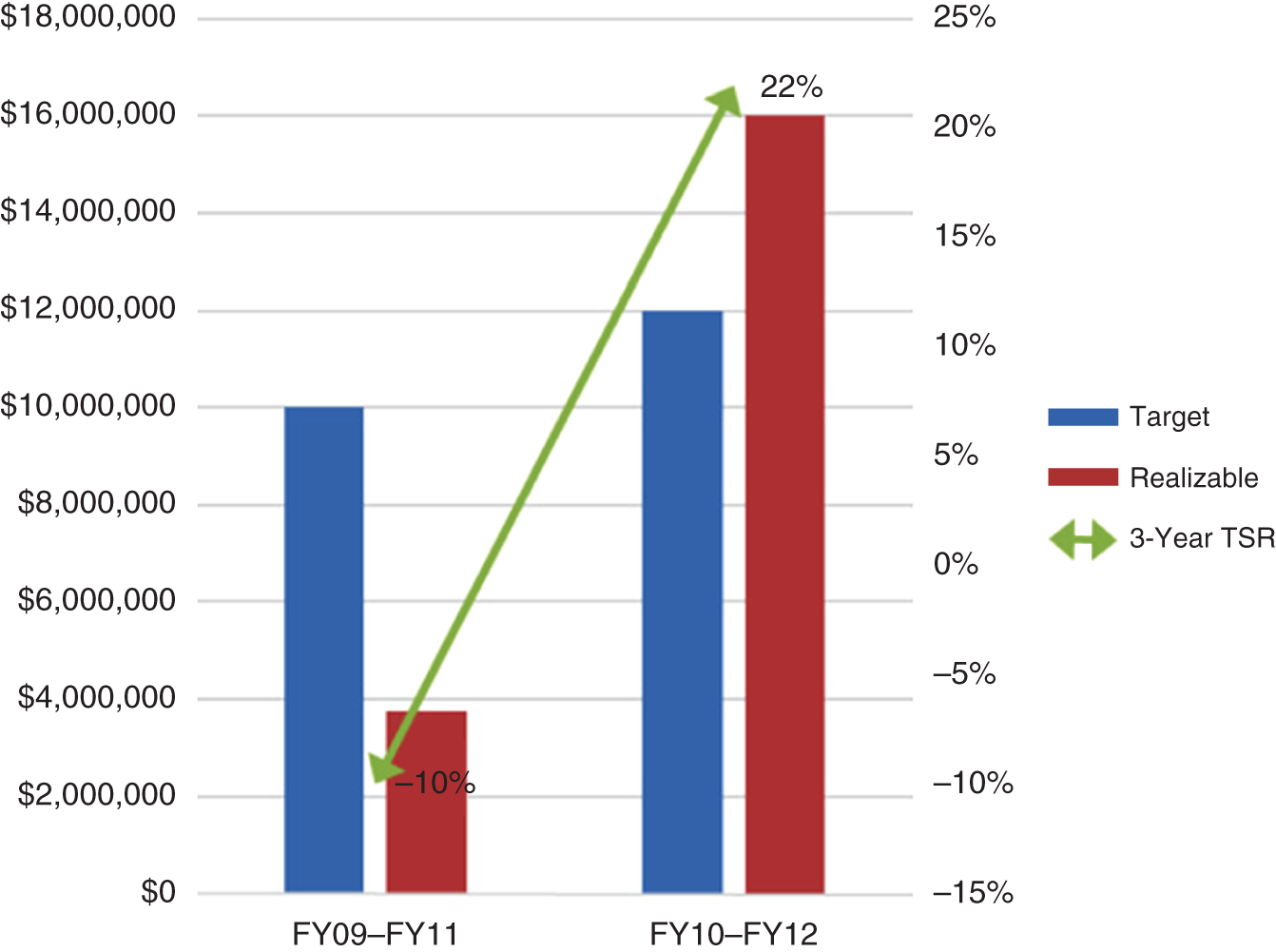
EXHIBIT 39.2 Target and Realizable Pay Versus Three-Year TSR (Total Shareholder Return)
Source: The Conference Board, “2013 Report on Supplemental Pay Disclosure.”

EXHIBIT 39.3 Relative Pay Versus Relative Performance
Source: Shareholder Value Advisors.
In this analysis, relative pay is plotted on the vertical axis against relative performance on the horizontal axis, and a regression trendline relating relative pay to relative performance is calculated (the dashed line). The slope of the trendline is a measure of incentive strength. It gives the change in relative pay associated with a one-unit change in relative performance. When relative pay and relative performance are plotted on a log scale, the slope of the trendline is the percent change in relative pay associated with a 1 percent change in relative performance. This is a measure of incentive strength that can be compared across companies without any need for size adjustment.
The graph provides three additional measures of pay effectiveness. The correlation of relative pay and relative performance is a measure of alignment. The intercept, which is where the trendline crosses the light-blue vertical axis, is the pay premium at zero relative performance, that is, the pay premium at peer group average performance. This pay premium, on the negative side, is a measure of retention risk. The more pay for average performance falls below average pay, the greater is the likelihood that a capable executive can find a better paying job. The pay premium, on the positive side, is a measure of shareholder cost. The more pay for average performance rises above average pay, the greater is the burden of shareholder cost. The third measure of pay effectiveness is the ratio of the slope to the correlation. This ratio is the ratio of relative pay variability to relative performance variability, and hence provides a measure of pay risk. When relative pay is much more volatile than relative performance, pay is likely to provide an incentive to take excessive risk.
This simple graph provides a very flexible and powerful framework for measuring and improving pay for performance. It can be used with mark-to-market pay10 that captures the incentive provided by changes in the value of unvested equity compensation or it can be used with grant date pay. It can be used with market measures of performance, such as TSR, where relative performance is relative TSR. It can also be used with operating measures of performance, such as operating return,11 where relative performance is operating return adjusted for either the company's ex-ante cost of capital or the average operating return of peer companies.
Exhibit 39.4 shows this analysis for Monsanto CEO Hugh Grant using mark-to-market pay data for the first nine years of his CEO tenure. In this graph, each data point represents cumulative pay and cumulative performance from the start of Grant's first year as CEO, 2004. The vertical axis is the natural logarithm of relative mark-to-market pay. The horizontal axis is the natural logarithm of (1 + relative TSR). The slope of the line, or what we call pay leverage, is 0.84. This means that 1 percent in relative shareholder wealth increases relative pay by 0.84 percent on average. The squared correlation is 48 percent. This means that relative performance explains 48 percent of the variation in relative pay over the nine measurement periods. The pay premium at peer group average performance, that is, zero relative TSR, is +63 percent. This means that Grant's pay, measured on a mark-to-market basis, is 63 percent above average when Monsanto's TSR matches the industry.

EXHIBIT 39.4 Relative Pay Versus Relative Total Shareholder Return
Source: Shareholder Value Advisors.
Mark-to-market pay for a period is cumulative pay with equity compensation valued at the end-of-period stock price (or vesting date stock price if earlier). Relative mark-to-market pay is mark-to-market pay for a period divided by cumulative market pay for period. Market pay is trendline grant date pay taking account of position, industry, and company size and adjusted for the expected accretion of equity compensation. For example, for Monsanto CEO Hugh Grant, the position is CEO, the industry is the materials industry group (GICS 1510), and company size is Monsanto's revenue size at the start of the nine-year period. We calculate market rates using company size at the start of the pay for performance analysis period rather than company size in each year of the analysis period. The expected accretion of equity compensation is the average percentage increase (for all company years in the database) in the value of equity compensation from date of grant through the end of the pay for performance analysis period.
Our calculation of market rates using initial, not current, sales and our use of expected, not actual, equity compensation values are both designed to provide a better definition of perfect pay for performance. We define perfect pay for performance as a pay plan that provides a perfect correlation of relative pay and relative performance with a zero-pay premium at peer group average performance. If we adjust market pay for annual sales growth, we build in the assumption that perfect pay requires pay increases for annual sales, not just relative TSR. If we use actual peer company mark-to-market pay, not grant date pay adjusted for expected accretion, we build in the assumption that perfect pay requires matching the peer companies' actual compensation for industry performance. Since the goal of perfect pay for performance is to pay for superior management performance, not industry performance, this makes no sense at all. It is appropriate, however, to say that perfect pay provides the expected accretion in equity compensation. Put another way, the expected future value of perfect pay needs to be competitive with the expected future value of market pay.
Relative TSR must take account of Monsanto's industry beta. A great deal of pay for performance analysis defines relative TSR as [(1 + TSR)/(1 + industry TSR)] – 1. This calculation assumes that the company's industry beta is 1.0, that is, a 1 percent change in industry shareholder wealth will increase company shareholder wealth by 1.0 percent. That's a pretty good assumption for the median company because the median company has an industry beta of 0.95, but a poor assumption for many other companies. When we look at S&P 1500 companies and use GICS industry groups as peer groups, we find that 20 percent of companies have industry betas greater than 1.65 while another 20 percent have industry betas below 0.25. For about 10 percent of S&P 1500 companies, the GICS industry group is not a meaningful peer group because the industry beta is zero or negative. Exhibit 39.5 shows that Monsanto's industry beta is 2.39.

EXHIBIT 39.5 Company Versus Industry Total Shareholder Return for Monsanto, Relative TSR = [(1 + TSR)/((1 + industry TSR)^2.38)] − 1
The Design Implications of the Measurement Analysis: Perfect Pay Plans
Once we develop a good way of measuring pay for performance, we can do two important things. We can ask, What is a perfect pay plan, that is, a plan that provides alignment of 1.0 with a zero pay premium at peer group average performance? And we can benchmark our pay for performance against our peers.
There is a simple performance share plan that provides perfect pay for performance. We can see the logic of the perfect performance share plan if we return to the “Good Early Performance” and “Bad Early Performance” scenarios we looked at in Exhibit 39.1. Exhibit 39.6 shows the same two scenarios with a critical modification in the calculation of grant shares. We now calculate grant shares using target pay, which is not market pay, but market pay adjusted for trailing relative performance. The exhibit now shows industry performance, which—adjusted to the beginning stock price—rises from $10 in year 0 to $15 at the end of year 5. We use industry performance to calculate relative return (= (stock price/beginning stock price × (1 + industry return)) – 1) and set target pay equal to market price × (1 + relative return). Adjusting for trailing relative performance eliminates the “performance penalty” in grant shares. In year 2, Good Early Performance and Bad Early Performance both get 91 grant shares even though the beginning stock price in Good Early Performance is $15 while the beginning stock price in Bad Early Performance is $7. Good Early Performance has a relative return of +36% (= (15/11) – 1), which raises target pay to $1,364. Dividing by the stock price of $15 gives grant shares of 91. Bad Early Performance has a relative return of –36% (= (7/11) – 1), which lowers target pay to $636 and grant shares to 91. Both scenarios now receive the same total number of shares, 423, and have the same ending wealth, $8,452.
EXHIBIT 39.6 Tying Target Pay to Trailing Relative Performance Eliminates Pay Differences for the Same Cumulative Performance
| Year | Year | Year | Year | Year | Year | |
| 0 | 1 | 2 | 3 | 4 | 5 | |
| Market pay | 1,000 | 1,000 | 1,000 | 1,000 | 1,000 | |
| Beginning stock × (1 + industry return) | 10 | 11 | 12 | 13 | 14 | 15 |
| GOOD EARLY PERFORMANCE | ||||||
| Stock price | 10 | 15 | 20 | 25 | 30 | 20 |
| Relative return (at beginning of year) | 0% | 36% | 67% | 92% | 114% | |
| Target pay (= market × (1 + relative return)) | 1,000 | 1,364 | 1,667 | 1,923 | 2,143 | |
| Grant shares (= target pay / BOY stock price) | 100 | 91 | 83 | 77 | 71 | |
| Cumulative shares | 100 | 191 | 274 | 351 | 423 | |
| Ending wealth | 8,452 | |||||
| BAD EARLY PERFORMANCE | ||||||
| Stock price | 10 | 7 | 6 | 5 | 8 | 20 |
| Relative return (at beginning of year) | 0% | −36% | −50% | −62% | −43% | |
| Target pay (= market × (1 + relative return)) | 1,000 | 636 | 500 | 385 | 571 | |
| Shares (= target pay / stock price) | 100 | 91 | 83 | 77 | 71 | |
| Cumulative shares | 100 | 191 | 274 | 351 | 423 | |
| Ending wealth | 8,452 |
Our use of target pay aligns cumulative pay and cumulative performance across the good and bad early performance scenarios, but it doesn't align relative pay with relative performance. Ending executive wealth is 169 percent of cumulative market pay even though ending shareholder wealth is only 133 percent of industry shareholder wealth. To align relative pay and relative performance, we need to use vesting to take out the industry component of the stock return. The way to do that is to make the vesting multiple equal to 1/(1 + the industry return from the date of grant). Exhibit 39.7 shows the calculation of the vesting multiples at the end of year 5. Vesting shares at the end of year 5 total 333. This makes ending executive wealth $6,667 (= 333 × $20), which in turn makes the relative pay ratio, 133% (= $6,667/$5,000), equal to the relative shareholder wealth ratio.
EXHIBIT 39.7 Making the Vesting Multiple Equal to 1 / (1 + Industry Return) Is the Third Component of the “Perfect” Pay Plan
| Year | Year | Year | Year | Year | Year | |
| 0 | 1 | 2 | 3 | 4 | 5 | |
| Market pay | 1,000 | 1,000 | 1,000 | 1,000 | 1,000 | |
| Beginning stock × (1 + industry return) | 10 | 11 | 12 | 13 | 14 | 15 |
| GOOD EARLY PERFORMANCE | ||||||
| Stock price | 10 | 15 | 20 | 25 | 30 | 20 |
| Relative return (beginning of year) | 0% | 36% | 67% | 92% | 114% | |
| Target pay (= market × (1 + relative return)) | 1,000 | 1,364 | 1,667 | 1,923 | 2,143 | |
| Grant shares (= target pay / BOY stock price) | 100 | 91 | 83 | 77 | 71 | |
| Industry return from grant to end of year 5 | 50% | 36% | 25% | 15% | 7% | |
| Year 5 vesting multiple (= 1 /(1 + industry return)) | 0.67 | 0.73 | 0.80 | 0.87 | 0.93 | |
| Vesting grant shares | 67 | 67 | 67 | 67 | 67 | |
| Cumulative vesting shares | 67 | 133 | 200 | 267 | 333 | |
| Ending wealth | 6,667 | |||||
| BAD EARLY PERFORMANCE | ||||||
| Stock price | 10 | 7 | 6 | 5 | 8 | 20 |
| Relative return (beginning of year) | 0% | −36% | −50% | −62% | −43% | |
| Target pay (= market × (1 + relative return)) | 1,000 | 636 | 500 | 385 | 571 | |
| Grant shares (= target pay / BOY stock price) | 100 | 91 | 83 | 77 | 71 | |
| Industry return from grant to end of year 5 | 50% | 36% | 25% | 15% | 7% | |
| Year 5 vesting multiple (= 1 /(1 + industry return)) | 0.67 | 0.73 | 0.80 | 0.87 | 0.93 | |
| Vesting grant shares | 67 | 67 | 67 | 67 | 67 | |
| Cumulative vesting shares | 67 | 133 | 200 | 267 | 333 | |
| Ending wealth | 6,667 |
Exhibit 39.8 shows the math behind the plan design, using target pay leverage of 1.0. Target compensation is market compensation adjusted for trailing relative performance, that is, target compensation = market compensation × (1 + relative TSR). This ensures that every grant reflects relative performance up to the time of grant. To achieve perfect pay for performance, the value of every grant must also reflect relative performance after the time of grant. This is accomplished by the performance share vesting. The vesting provisions need to take out the industry component of the stock return so that the vesting stock value only reflects relative TSR from the date of grant forward. This is accomplished by making the vesting multiple inversely proportional to the industry return, as Exhibit 39.8 shows.12 We can see that the vesting stock value from any year's grant is equal to market compensation for the year adjusted for relative performance over the CEO's entire tenure. A final component of the perfect pay for performance plan is that any nonperformance pay is treated as a draw against the value of the performance shares.
EXHIBIT 39.8 The Math Behind the Perfect Performance Share Plan
| Target compensation | = | market compensation × (1 + relative TSR from start of CEO tenure to date of grant) |
| Performance shares granted | = | target compensation / stock price |
| Vesting multiple | = | 1 / (1 + industry TSR from date of grant) |
| Value of performance shares granted | = | stock value × vesting multiple |
| = | grant value × (1 + TSR from date of grant) × 1 / (1 + industry TSR from date of grant) | |
| = | grant value × (1 + relative TSR from date of grant) | |
| = | market compensation × (1 + relative TSR from start of CEO tenure to date of grant) × (1 + relative TSR from date of grant) | |
| = | market compensation × (1 + relative TSR from start of CEO tenure to end of measurement period) |
The perfect pay for performance plan helps us see that three widely accepted pay-plan features undermine pay for performance. First is the concept of fiftieth percentile pay regardless of past performance. The design of the perfect pay for performance plan shows that the concept of competitive pay regardless of past performance needs to be replaced by the concept of competitive pay for average performance. Second is the concept that vesting should leverage operating performance. The design of the perfect pay for performance plans shows that the role of vesting is to take out the industry component of the stock return, not to leverage operating performance. Third is the concept that nonperformance pay is an independent entitlement. Nonperformance pay, as well as any drawdown of the performance share value, must be treated as a draw against the value of the performance shares, not a separate entitlement.
If market compensation is constant, the perfect pay for performance pay plan, with pay leverage of 1.0, makes cumulative pay equal to cumulative market pay plus a fixed percentage of the cumulative dollar excess return, which may be negative. Exhibit 39.9 shows the derivation of the sharing formula.13
This expression for cumulative perfect pay shows that the perfect performance share plan integrates the two strands of executive pay history. It provides competitive pay and fixed sharing, so it is able to limit retention risk while still providing strong incentives.
Remarkably, there are two other perfect plans that also imply that perfect pay is equal to cumulative market compensation plus a fixed share of an excess return. One is the perfect fee structure for investment managers developed by Don Raymond, the chief investment strategist of the Canada Pension Plan Investment Board.14 The second is the Dynamic Incentive Account developed by finance professors Alex Edmans and Xavier Gabaix. Their paper was named best paper of 2009 by the Financial Research Association and was a finalist for the McKinsey/HBR management innovation of the year award.15
EXHIBIT 39.9 Perfect Pay Calculation: Derivation of Sharing Formula
| Value of performance shares granted | = | market compensation × (1 + relative TSR from start of CEO tenure to end of measurement period) |
| Cumulative perfect pay | = | cumulative market compensation × (1 + relative TSR) |
| = | initial grant shares × initial grant price × CEO years × (1 + relative TSR) | |
| = | initial grant shares × initial grant price × CEO years + initial grant shares × initial grant price × CEO years × relative TSR) | |
| = | cumulative market compensation + (CEO years × initial grant shares × initial grant price × relative TSR) | |
| = | cumulative market compensation + (CEO years × initial grant shares × [shares outstanding / shares outstanding] × initial grant price × relative TSR) | |
| = | cumulative market compensation + (CEO years × [initial grant shares / shares outstanding] × shares outstanding × initial grant price × relative TSR) | |
| = | cumulative market compensation + (CEO years × [initial grant shares / shares outstanding] × dollar excess return) | |
| = | cumulative market compensation + sharing percentage × dollar excess return |
Benchmarking Pay for Performance
Pay alignment, performance adjusted cost, that is, the pay premium at industry average performance, and relative risk are well suited to benchmarking and ranking because they can be compared across companies without any need for industry or size adjustment and there is a high level of agreement about the ordinal ranking of each dimension. Few would dispute that more alignment is better than less alignment, that a larger positive pay premium is worse than a smaller positive pay premium, or that a relative risk ratio well above 1.0 is worse than relative risk ratio closer to 1.0. By contrast, there is not a lot of agreement about an ordinal ranking of pay leverage. Some people feel that pay leverage of 1.25 is better than pay leverage of 0.75 while others feel that pay leverage of 1.25 is worse than pay leverage of 0.75.
Exhibit 39.10 shows the prevalence of pay for performance problems among S&P 1500 CEOs over the 10 years 2007–2016. The four problems are low alignment, where relative TSR explains less than 50 percent of the variation in relative pay, high pay risk, where relative pay variability is 50 percent or more greater than relative performance variability, high retention risk, where the pay premium at industry average performance is –33 percent (or below), and high cost, where the pay premium at industry average performance is 50 percent or more. Eighty-seven percent of companies have at least one of these four problems.
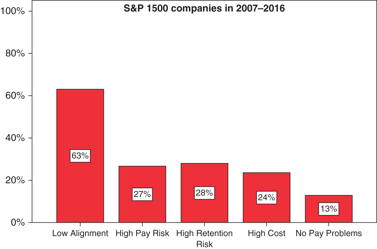
EXHIBIT 39.10 Problems in Achieving the Three Basic Pay Objectives for CEOs
Executive Pay Has a Big Impact on Shareholder Wealth
It's easy for directors to rationalize high pay for top management. High pay limits the risk of losing the top management team and the cost of overpayment is trivial for the average shareholder. We mentioned earlier our 2013 research showing that 10 CEOs received $40+ million just as a result of the additional shares and lower exercise prices they received as a result of stock price declines. One of the 10 is Edward Whitacre Jr. of AT&T whose 2004 stock value was increased by $41 million just from the additional shares and lower exercise prices awarded over the prior five years due to stock price declines. In 2004, AT&T had 3.3 billion shares outstanding, so Whitacre's extra pay from poor performance was less than a penny per share after tax ($0.0076 per share). It's easy to rationalize that trivial cost as a small price for shareholders to pay to ensure the retention of their CEO.
This is a very misguided view. The negative impact of high top 5 pay (relative to performance) on shareholder wealth is much greater than the direct after-tax cost of the top 5's excessive pay. Moreover, top 5 pay leverage has a statistically and economically significant impact on future shareholder returns. Directors should use models of the shareholder wealth impact of pay dimensions to evaluate their management pay program and to benchmark their programs against peers.
A working paper (Available at http://www.valueadvisors.com/publications.htm) on “Top 5 Compensation Cost, Holdings & Future Stock Returns” by Professor David Young of INSEAD and me shows that 10-year measures of pay leverage and the pay premium at industry average performance have statistically and economically significant effects on future 1-, 3-, and 5-year excess returns. We also find that more current proxies for pay leverage and the pay premium at industry average performance—computed with only three years of historical data—have even bigger effects on future 1-, 3-, and 5-year excess returns. The data source for our analyses is Standard & Poor's Execucomp database. Execucomp begins in 1992, so our first calculation of 10-year pay leverage ends in 2001. This is also our first base year for measuring future returns. The 2018 Execucomp database, with pay data through 20, allows us to test the impact of pay factors on 16 annual returns, 14 3-year returns, and 12 5-year returns.
The dependent variable in each regression is ln((1 + TSR)/(1 + expected TSR based on a four-factor Fama-French model). We measure TSR beginning and ending four months after fiscal year-end to ensure that the pay factor data in our model is known to investors at the start of the return measurement. We use a stepwise multiple regression to help us evaluate three basic choices in measuring the dimensions of pay for performance: (1) Should we use pay for performance measures for the CEO or the top 5? (2) Should we use pay for performance measures based on mark-to-market pay or grant date pay? (3) Should we measure pay for performance using relative TSR or relative operating return? We test these alternatives after taking account of momentum (i.e., prior relative return) and time (i.e., dummy variables for each year).
For brevity, we will focus on our model of 3-year returns using 10-year measures of pay leverage and the pay premium at industry average performance. In that model, momentum and time explain 3.8 percent of the variation in ln(1 + 3-year excess return) across a sample of 8,026 cases. After momentum and time, the first and second most significant explanatory variables are top 5 mark-to-market (MtM) pay leverage versus relative TSR and the top 5 pay premium at industry average performance, measured against relative operating return. Together, these two variables explain an additional 0.6 percent of the variance in ln(1 + 3-year excess return). A two-standard-deviation difference in pay leverage increases the 3-year excess return by 4.5 percentage points and a two-standard-deviation difference in the pay premium at industry average performance reduces the 3-year excess return by 7.1 percentage points; 20 percent of S&P 1500 companies have predicted 3-year excess returns from pay leverage and the pay premium at industry average performance that exceed 4 percentage points, positive or negative.
Directors can use this model to benchmark their pay program against their peers. Exhibit 39.11 shows a ranking of software companies (GICS industry 451030) by predicted excess return. Some of the highly ranked companies, such as Intuit, the developer of QuickBooks, have substantial pay premiums, but the negative effect of their pay premium is offset by their high pay leverage. Some of the low-ranked companies, such as SalesForce, have substantial pay leverage, but the positive effect of their pay leverage is offset by their extremely high pay premium at industry average performance.
EXHIBIT 39.11 Ranking of Software Companies by Predicted Excess Return
| Company | Predicted Excess Return | Mark-to-Market Pay Leverage | Grant Date Pay Premium at Industry Average Performance |
| MICROSOFT CORP | 0.08 | 2.42 | 0.00 |
| SYNOPSYS INC | 0.08 | 2.39 | 0.00 |
| FAIR ISAAC CORP | 0.07 | 2.09 | 0.00 |
| ADOBE SYSTEMS INC | 0.06 | 2.40 | 0.29 |
| TYLER TECHNOLOGIES INC | 0.04 | 1.26 | 0.00 |
| INTUIT INC | 0.03 | 2.24 | 0.63 |
| MANHATTAN ASSOCIATES INC | 0.03 | 0.88 | 0.00 |
| ANSYS INC | 0.02 | 1.12 | 0.19 |
| ACI WORLDWIDE INC | 0.02 | 0.65 | 0.00 |
| BLACKBAUD INC | 0.02 | 2.14 | 0.76 |
| MONOTYPE IMAGING HOLDINGS | 0.01 | 0.69 | 0.18 |
| CADENCE DESIGN SYSTEMS INC | 0.01 | 0.86 | 0.26 |
| SMITH MICRO SOFTWARE INC | 0.01 | 0.19 | 0.00 |
| AWARE INC | 0.01 | 0.16 | 0.00 |
| TIVO CORP | 0.01 | 0.95 | 0.38 |
| CITRIX SYSTEMS INC | 0.00 | 0.97 | 0.40 |
| MICROSTRATEGY INC | −0.01 | 0.37 | 0.26 |
| BOTTOMLINE TECHNOLOGIES INC | −0.01 | 0.32 | 0.28 |
| PTC INC | −0.02 | 0.28 | 0.38 |
| ELECTRONIC ARTS INC | −0.02 | 1.47 | 0.98 |
| ASPEN TECHNOLOGY INC | −0.02 | 1.57 | 1.05 |
| AUTODESK INC | −0.03 | 0.00 | 0.47 |
| EBIX INC | −0.04 | 0.33 | 0.78 |
| SALESFORCE.COM INC | −0.06 | 0.88 | 1.31 |
| ULTIMATE SOFTWARE GROUP INC | −0.09 | 0.33 | 1.41 |
Directors Need to Ensure That They Themselves Have Strong Incentives to Increase Shareholder Value
Director pay design is typically guided by the same concepts as executive pay design, that is, target competitive position and target percent of pay at risk, and shows a similar prevalence of low alignment and other pay problems. Exhibit 39.12 shows the prevalence of pay for performance problems among S&P 1500 directors over the 10 years 2007–2016. Low alignment is almost as common among directors as CEOs (60% vs. 63%). High pay risk is less common among directors (18% vs. 27%) as is high retention risk (13% vs. 28%) while high cost is more common (31% vs. 24%). Eighty-two percent of companies have at least one director pay problems (vs. 87% of companies with at least one CEO pay problem).
In the distant past, directors had little need to worry about director pay design because their stock ownership provided much stronger incentives than their director pay. Over time, there has been a dramatic change in director incentives caused by a sharp decline in stock ownership and a big increase in director pay. In a 2018 study of “The Evolution of Executive Pay Policy at General Motors 1918–2008,” David Young and I found a dramatic decline in director incentives from stock ownership between 1947 and 1977 (O'Byrne and Young, 2017). To measure the relative strength of stock versus pay incentives, we compared the expected annual return on the director's stock with the director's fee for board service. In 1947, the median director owned $1.65 million in stock and received an annual director's fee of $900. Assuming a 10 percent expected return on the stock, the expected return on the median director's stock was 183 times the director's pay for board service. Put another way, the director's fee made up for the loss of the expected return on the director's stock for a total of two days. This balance gave the director a very strong financial incentive to develop executive pay plans that increased shareholder wealth. In 1977, the year in which the GM board dropped the single pool sharing concept that had guided GM incentive pay since 1992, the median director owned $34,000 in stock and received an annual director's fee of $47,000. Assuming a 10 percent expected return on the stock, the expected return on the median director's stock was 7 percent of the director's pay for board service. Put another way, the director's fee made up for the loss of the expected return on the director's stock for almost 14 years. This balance gave the director a very strong financial incentive to promote higher pay for management and directors regardless of its impact on shareholders.

EXHIBIT 39.12 Problems in Achieving the Three Basic Pay Objectives for Directors
The first step in board oversight of executive pay should be the design of a director pay plan that provides strong incentives to increase shareholder wealth.
Institutional Investors Don't Do a Good Job on Say on Pay
In theory, institutional investors should have strong financial incentives to promote better executive and director pay. In practice, there is substantial evidence that the largest institutional investors devote few resources to monitoring their portfolio companies and that the quality of their Say on Pay decisions is no better than that of the average investor.
A study by law professors Lucian Bebchuk and Scott Hirst (2019) shows that the stewardship staffs of the three largest institutional investors—BlackRock, State Street, and Vanguard—are so modest in size that they account for less than 0.2 percent of the management fees charged by these funds.
Exhibit 39.13 shows a measure of Say on Pay (SOP) voting quality for the ten largest asset managers and the average investor (the dotted line). The measure is designed to answer two questions: Is SOP voting informed? And is it fair to shareholders? To calculate our measure of voting quality, we first develop a custom pay equity measure for each asset manager using 100–300+ votes for the manager. The custom pay equity measure tells us the weight the asset manager puts on three measures of CEO pay equity (i.e., pay equity vs. relative TSR, pay equity vs. relative ROIC, and pay equity vs. other members of the top 5). We then use this custom pay equity measure to ask two questions: Is the manager's SOP voting informed by objective pay equity measures, that is, how correlated is the manager's SOP voting with its custom pay equity measure? And is the manager's SOP voting fair to shareholders, that is, how often does the manager vote “no” on CEOs who are 100+ overpaid based on the manager's custom pay equity measure? Our voting quality measure is the average of alignment (r-sq) with pay equity and the percent “no” vote.
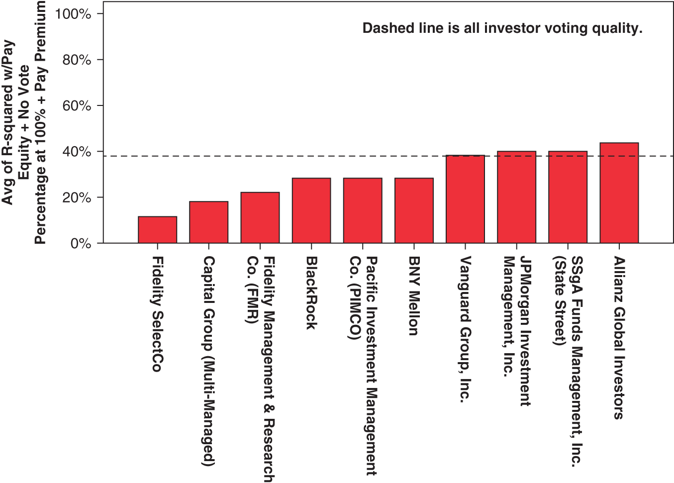
EXHIBIT 39.13 Voting Quality at the 10 Largest Funds
Our voting quality measure ranges from 0 percent to 100 percent. In a 2017 study of 213 funds, Mark Van Clieaf and I found that the voting quality of the best fund, 55.9 percent for West Fargo, was almost 50 percent better than the voting quality of the average investor, 37.8 percent (O'Byrne, 2018). Exhibit 39.13 shows that SOP voting quality is only slightly better than the average investor at State Street and Vanguard and considerably worse at BlackRock.
ISS Doesn't Do a Good Job for Institutional Investors
It makes sense for institutional investors to seek economies of scale in proxy voting analysis. In theory, the dominant proxy advisor, Institutional Shareholder Services (ISS), can help institutional investors achieve more effective and cost-effective oversight of executive and director pay. In practice, ISS has done little to advance compensation measurement or pay design.
ISS uses three measures to assess pay for performance: relative degree of alignment (RDA), multiple of median (MOM), and pay-TSR alignment (PTA). RDA takes account of relative pay and relative TSR but the actual measure ISS uses, the difference between a company's pay percentile and its TSR percentile, is a poor proxy for the correlation of relative pay and relative TSR. MOM is the ratio of the CEO's pay to median CEO pay without any adjustment for performance. This is an endorsement of competitive pay policy, which is a major cause of the misalignment of relative pay and relative performance, as we saw above. PTA is a measure of alignment with gross return: “The concept is simple: company pay and TSR trends to determine whether shareholders' and executives' experiences are directionally aligned.” But this makes no sense. Relative pay should be aligned with relative performance, not gross pay with gross performance.
In a 2012 study,16 I compared the ISS measures with pay leverage, pay alignment, and the pay premium at peer group average performance across a sample of 15,860 5-year periods for S&P 1500 companies, and found that RDA had correlations of –0.02 with pay leverage, –0.01 with pay alignment, and –0.45 with the pay premium at peer group average performance; PTA had correlations of 0.02 with pay leverage, 0.02 with pay alignment, and 0.10 with the pay premium at peer group average performance, and MOM had a correlation of 0.46 with the pay premium at peer group average performance. These correlations show that the ISS measures capture 21 percent (= 0.46 × 0.46) of the variation in one of the three pay for performance dimensions—performance-adjusted cost—but less than 1 percent of the variation in other two: pay leverage and pay alignment.
The fact that ISS continues to use these poorly designed measures is a sad testament to the limited compensation knowledge of the major institutional investors in the ISS client base. ISS clients don't seem to realize that the measures capture nothing but cost and don't voice complaints that would motivate ISS to improve the measures.
Conclusion
The key responsibility of the board in overseeing executive pay is to ensure that the company's executive pay program achieves the three basic objectives of executive pay: provide strong incentives to increase shareholder value, retain key talent, and limit the cost of executive pay to levels that maximize the wealth of existing shareholders. To effectively discharge this responsibility, the board needs meaningful measures of incentive strength and performance-adjusted cost, such as measures of pay leverage, relative pay risk, pay alignment, and the pay premium at peer group average performance. This chapter shows how these measures can be calculated, how they can be used to understand the pay design needed to achieve perfect pay for performance, and why the measures commonly used for board oversight—percent of pay at risk and competitive position—are very poor proxies for incentive strength and performance-adjusted cost.
The perfect performance share plan highlights three major shortcomings of current executive pay practice. First, the concept of fiftieth percentile pay regardless of past performance: This must be replaced by the concept of fiftieth percentile pay for average performance, not any performance. Second, the concept that vesting should leverage operating performance: This must be replaced by the concept that vesting should take out the industry component of the stock return. Third, the concept that nonperformance pay is an independent entitlement: This must be replaced by the concept that nonperformance pay is a draw against the value of the performance shares, not a separate entitlement. Given the prevalence of these bad practices, it is not surprising that pay-for-performance problems are common among S&P 1500 CEOs: 24 percent of CEOs show high pay, 27 percent show high pay risk, 63 percent show low alignment, 28 percent show high retention risk, and 87 percent show at least one of these three problems.
About the Author

Stephen F. O'Byrne is president and cofounder of Shareholder Value Advisors Inc., a consulting firm that helps companies increase shareholder value through better performance measurement, incentive compensation, and valuation analysis. His work on measuring the strength and cost-efficiency of top management incentives has been published in the Harvard Business Review, the Journal of Investing, Conference Board Director Notes, the Journal of Applied Corporate Finance, and the WorldatWork Journal. He is the coauthor, with Professor David Young of INSEAD, of EVA and Value-Based Management. He was previously head of the compensation consulting practice at Stern Stewart & Co. and a principal in the executive compensation practice at Towers Perrin.
Notes
- 1. The other two objectives are “support the achievement of Dow's vision and strategy” and “create ownership alignment with stockholders.” Dow Chemical 2015 proxy, p. 27.
- 2. Economic value added, or EVA, is a widely used term for economic profit. It's a trademark of Stern Stewart & Co., a consulting firm.
- 3. John C. Baker, “Incentive Compensation Plans for Executives,” Harvard Business Review 15, no. 5 (Autumn): 44–61.
- 4. General Motors proxy statement, April 17, 1948, p. 8.
- 5. General Motors proxy statement, April 15, 1977, p. 36.
- 6. Johnson & Johnson 2015 proxy, p. 36.
- 7. Stephen F. O'Byrne and E. Mark Gressle, “How ‘Competitive Pay’ Undermines Pay for Performance (and What Companies Can Do to Avoid That),” Journal of Applied Corporate Finance 25, no. 2 (Spring 2013): 26–38. Median S&P 1500 stock volatility is 0.4.
- 8. The Conference Board Working Group on Supplemental Pay Disclosure, “Supplemental Pay Disclosure: Overview of Issues, Proposed Definitions, and a Conceptual Framework,” The Conference Board (2013).
- 9. Exxon Mobil 2015 proxy, p. 48.
- 10. Mark-to-market pay for a measurement period is the sum of (1) salary, bonus, and other compensation; (2) the end of period value of equity compensation granted during the period; (3) the end of period value of cash long-term incentive awards made during the period; and (4) the change in pension value during the period. The end of period value of equity compensation is based on the stock price at the end of the period and, for performance shares, estimated vesting multiples. The end of period value of cash long-term incentive awards is based on target award values and estimated vesting multiples. Estimated vesting multiples for performance share grants and cash long-term incentive awards are based on relative TSR versus the GICS industry group, assuming a common vesting schedule (i.e., threshold vesting of 50 percent at twenty-fifth percentile performance, target vesting of 100 percent at fiftieth percentile performance, and maximum vesting of 200 percent at seventy-fifth percentile performance). Maximum vesting is less than 200 percent if the company reports a lower maximum award. Mark-to-market pay is similar to what others call realizable pay.
- 11. Operating return is total return with estimated future growth value. Market enterprise value = capital + EP/WACC + future growth value where EP is economic profit and WACC is the weighted average cost of capital. Operating value = capital + EP/WACC + predicted future growth value where future growth value is predicted from operating drivers such as R&D, advertising, sales growth, EBITDA growth, and sales growth × EP margin. Operating return = (change in operating value + future value of free cash flow)/beginning operating value. Relative operating return measured against ex-ante cost of capital is [(1 + operating return)/(1 + WACC)^years] − 1. Relative operating return measured against ex-post peer performance is [(1 + operating return)/(1 + peer group operating return)] −1.
- 12. This assumes the industry beta is 1.0. If the industry beta is not 1.0, the vesting multiple is 1/((1 + industry TSR)^beta).
- 13. Cumulative perfect pay (with leverage of 1.0) = cumulative market pay × (1 + relative TSR) = cumulative market pay + cumulative market pay × relative TSR; cumulative market pay × relative TSR = years × initial grant shares × initial grant price × relative TSR = years × initial grant shares × [shares outstanding/shares outstanding] × initial grant price × relative TSR = [years × initial shares/shares outstanding] × [shares outstanding × initial grant price × relative TSR] = sharing percentage × aggregate excess return.
- 14. Donald M. Raymond, “Paying (Only) for Skill (Alpha),” CFA Institute Conference Proceedings Quarterly, June 2008.
- 15. Alex Edmans, Xavier Gabaix, Tomasz Sadzik, and Yuliy Sannikow, “Dynamic CEO Compensation,” Journal of Finance LXVII, no. 5 (October 2012).
- 16. Stephen F. O'Byrne, “Assessing Pay for Performance,” Conference Board Director Notes 3, no. 19 (October 2011): 6.
References
- Bebchuk, Lucian, and Scott Hirst. 2019. “Index Funds and the Future of Corporate Governance: Theory, Evidence and Policy,” available at ssrn.com, abstract = 3282794.
- O'Byrne, Stephen F., and David Young, “Top 5 Compensation, Cost, Holdings & Future Stock Returns,” working paper available at www.valueadvisors.com/publications.htm.
- O'Byrne, Stephen F. 2018. “Say on Pay: Is It Needed? Does It Work?” Journal of Applied Corporate Finance, Winter 2018.
- O'Byrne, Stephen F., and S. David Young. 2017. “The Evolution of Executive Pay Policy at General Motors 1918–2008,” Journal of Applied Corporate Finance, Winter 2017.