
So far, we have covered a number of topics for various kinds of software and hardware exploitation. In this chapter, we shift our attention to one of the other core components in any IoT device architecture, communication.
Communication is the key component for any IoT architecture and it is responsible for devices talking to each other and sharing and exchanging data. The communication can either happen through a wired or wireless medium. In this and the next chapter, we cover various types of wireless communication technologies and explore software defined radio.
We start by understanding the concept of wireless communications. Wireless communications are the core component that IoT devices need to talk with each other. The effective range of wireless technologies spans from an extremely small distance to a few miles.
In this and the next chapter, we cover some wireless technologies, including topics such as software defined radio (SDR), BLE, and ZigBee. However, we won’t be going into the concepts of electromagnetic theory and the nitty-gritty of wireless technologies or digital signal processing.
Anyone who is reading this book will most certainly have experienced a form of wireless communication with the many devices that we are surrounded with. Be it controlling a television with a remote, or accessing the Internet using Wi-Fi or syncing your smart wearable wristband to your smartphone, all of this is done via one or the other forms of wireless communication technologies.
Even if you have never worked with radios before, you will find this chapter fascinating, practical, and extremely actionable. You might have used FM radio in your early days or have seen your parents use it. The problem with FM radio or any similar medium is the limitation of tuning to an extremely narrow range of functionalities and performing a specific set of actions programmed by the developer initially.
Imagine the power you would have if you could build and use a radio that has an extremely large frequency range and you could change its functionality as you wish without touching the hardware at all. That is what SDR does. SDR allows you to implement radio processing functionalities that otherwise would have needed hardware implementation to be performed with the use of software.
With this basic foundational knowledge of SDR, let’s look into what these are exactly, how to implement them, and finally how to use them for our IoT security and exploitation research.
Hardware and Software Required for SDR
Before we begin looking into SDR, here’s a list of the tools that we will be using in this chapter:
- 1.
GQRX
- 2.
GNURadio
- 1.
RTL-SDR
Software Defined Radio
By now, you will already have a lot of questions about SDR: How do these devices function? How we can create our own? We will take one step at a time, and try to understand the underlying principles of SDR first, and then move to further details.
I’ll start with an example. Imagine you are working on one of your IoT security penetration testing engagements and you have been given a wireless doorbell to pentest. You have tested all the hardware using the previous techniques we have discussed and now you need to look at the radio aspect. You look up the FCC ID of the device and find out that it communicates over 433 MHz. One of the things you can do is get a 433 MHz receiver to analyze the device’s radio properties and the kind of data it is transmitting. However, there is one limitation of this: What if the device transmits at 436 MHz or the next device you pentest transmits at 355 MHz?
A better solution to approach this particular scenario is to work with SDR, which will allow you to modify the radio frequency that you’re listening to and the way you decode the signal based on whichever device you are assessing. Therefore, you no longer need different hardware for different devices, but rather a combination of a single hardware and software utility that will allow you to make changes according to your requirements.
This is exactly what SDR allows you to achieve: You can modify the processing done by the radio component depending on your needs.
Setting Up the Lab
The first thing we should do, before we jump into analyzing frequencies and looking at all the finer details, is to set up our lab environment for the SDR. I strongly recommend setting up the lab for all the SDR exercises on Ubuntu, as other platforms might not be as easy to set up. In addition, Ubuntu is better able to work with advanced concepts when we go deeper later on.
- 1.
GNURadio.
- 2.
GQRX.
- 3.
Rtl-sdr utilities.
- 4.
HackRF tools.
You will also need access to SDR hardware. There are a number of options to choose from and all of them have their own benefits. However, to keep things simple at the start, I have chosen the RTL-SDR, which is an extremely inexpensive ($20) piece of hardware that will allow us to perform a number of our SDR-related exercises. Later on, in this chapter, I also show how we can use HackRF for additional radio exploitation.
One of the limitations of RTL-SDR is that it will only allow you to sniff and look at various frequencies, and not actually transmit your own data. Even though there are hardware modifications available for RTL-SDR with which you can transmit data, for those purposes, I would strongly recommend getting a tool such as HackRF.
Installing Software for SDR Research
As mentioned earlier, I recommend performing all of the SDR exercises on an Ubuntu machine. I would also recommend you have Ubuntu as your base operating system and not do these exercises inside a VM, unless that’s the only option.
SDR 101: What You Need to Know
Before we move further, we need to go through the many underlying concepts that will come into use once we start working with SDR. In this section, we cover some of the extremely basic but important topics that you need to understand before doing anything significant in SDR.
Let’s start with a very simple example—communication through a Wi-Fi router. This means the Wi-Fi router is emitting signals in the air that a laptop is able to pick up through its Wi-Fi chipsets, for example. The Wi-Fi router in this case is the transmitter, and the wireless chip inside the laptop is the receiver.
If we go into finer detail, the data that need to be transmitted from the Wi-Fi router are being modulated with a carrier signal of 2.4 GHz. These data are then being passed through the air (transmitting medium) and received on the other end. Once is the data are received, they are decoded and the final data are obtained from the signal. The modulation process is essential for a number of purposes including noise reduction, multiplexing, working with various bandwidths and frequencies, cable properties, and so on.
As you might have realized, in a modulation, the baseband signal, which is considered the main information source, is carried by a higher frequency wave called the carrier signal. Based on the properties of the carrier signal and the type of modulation being used, the properties of the final signal, which travels through the air, change.
Analog modulation: Amplitude, frequency, SSB, and DSB modulation.
Digital modulation: Frequency Shift Keying (FSK), Phase Shift Keying (PSK), and Quadrature Amplitude Modulation (QAM).
Amplitude modulation
Frequency fodulation
Phase modulation
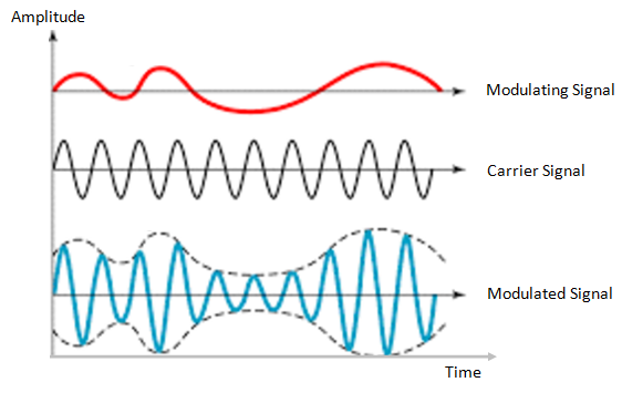
Amplitude Modulation
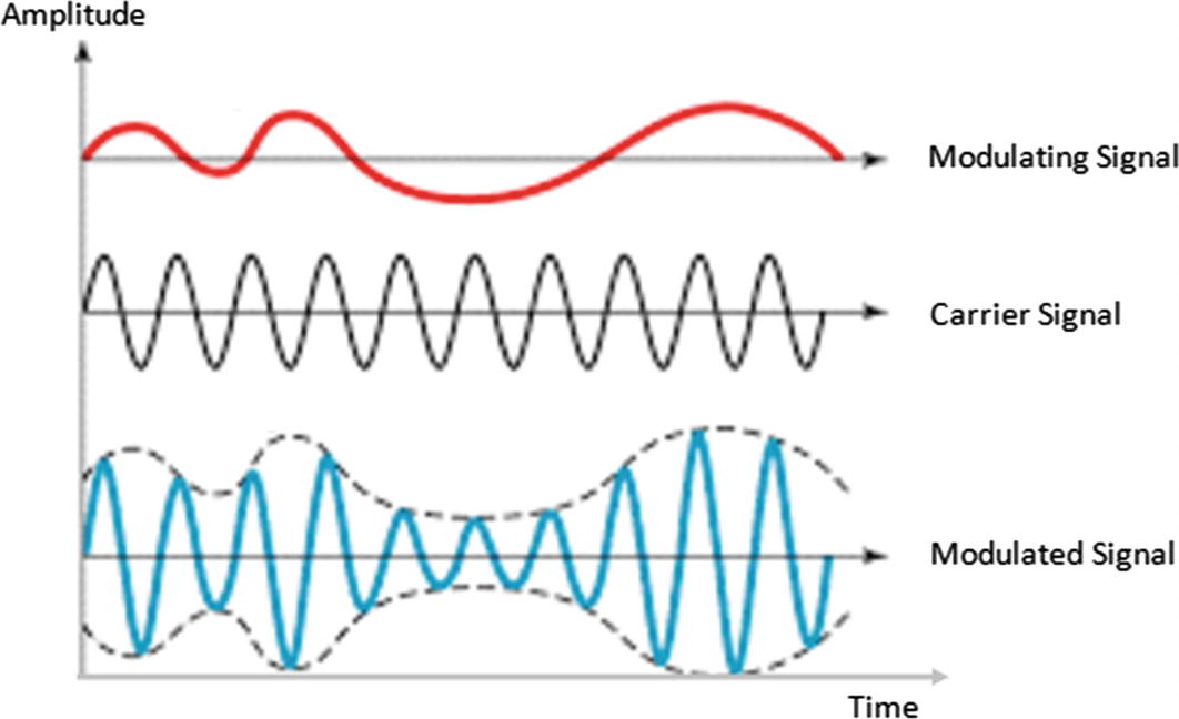
Amplitude modulation in action (Source: https://electronicspost.com/wp-content/uploads/2015/11/amplitude-modulation1.png )
In Figure 9-1, the modulating signal is being modulated with the carrier signal to produce the final modulated signal. Notice how the amplitude of the final modulated signal is the result of the combined amplitudes of the modulating and carrier signals.
Frequency Modulation
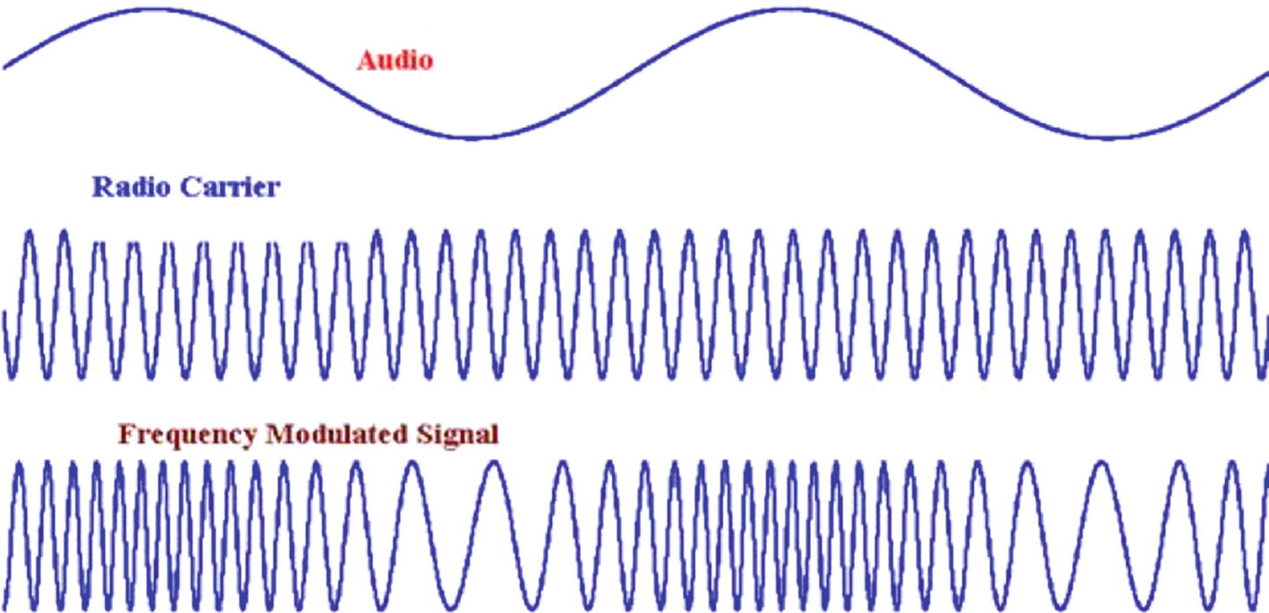
Frequency modulation. (Source: http://www.g4prs.org.uk/ )
Phase Modulation

Phase modulation in progress (Source: http://semesters.in/basics-of-angle-modulation-electronics-engineering-notes-pdf-ppt/ )
Common Terminology
Let’s now look at some of the common terminology you might encounter while doing SDR security research. I keep it brief to provide an introduction and understanding of what the different components are without going into highly technical details relating to digital signal processing at this stage.
Transmitter
A transmitter is a component in the radio system that generates an electric current to be transmitted. It is an electronic source that emits the data that needs to be modulated.
Analog-to-Digital Converter
As the name suggests, the analog-to-digital converter (ADC) simply converts analog signals to their digital counterparts. This is done by taking note of the value at periodic intervals of time (sample rate) and then plotting a waveform around it. Remember, most of the real-world data that you collect are analog data, whereas the data that computers understand are digital data.
Because computers can only understand digital data, you will find the ADC component in almost all the SDR hardware tools that you use. The exact opposite of an ADC is a digital-to-analog converter.
Sample Rate
The sample rate is the number of samples measured per second of a given signal. It simply means the number of times we are taking note of the values in the signal in one single second. Ideally, the sample rate of any signal to be reproduced should be at least twice the value of the frequency of that signal.
Sample rate is calculated in millions of samples per second (MSPS). For instance, 802.11 needs at least 20 MSPS of bandwidth to work.
Fast Fourier Transform
During your entire SDR security research journey, you will hear the term fast Fourier transform (FFT) a number of times. FFT is an improved and faster version of discrete Fourier transform. It is an algorithm that helps us isolate different frequencies by changing the plot from time domain to frequency domain. This is also something we cover later in this chapter in more detail.
Bandwidth
Bandwidth is the frequency range that is required to carry a signal. In other words, the distance between the highest and lowest frequencies carried by a signal is referred to as bandwidth.
Wavelength
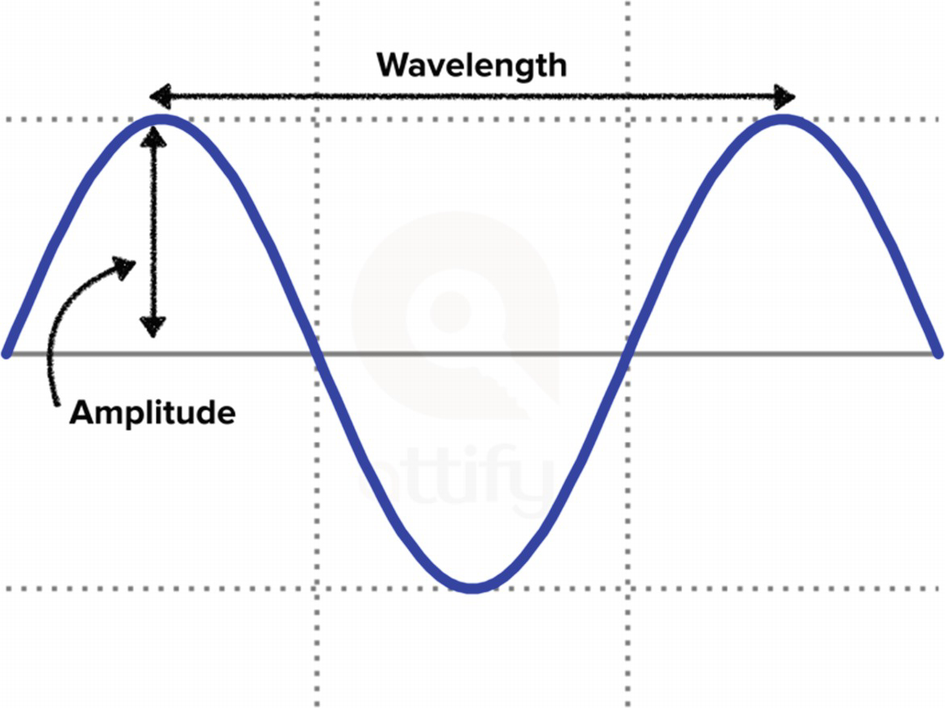
Waveform illustrating wavelength and amplitude in a signal
Frequency
Frequency simply means how frequently an event happens. In the case of radio, it means the number of cycles of a wave for every given second or the rate of oscillation of waves. This is also inversely proportional to the wavelength and is measured in Hertz.
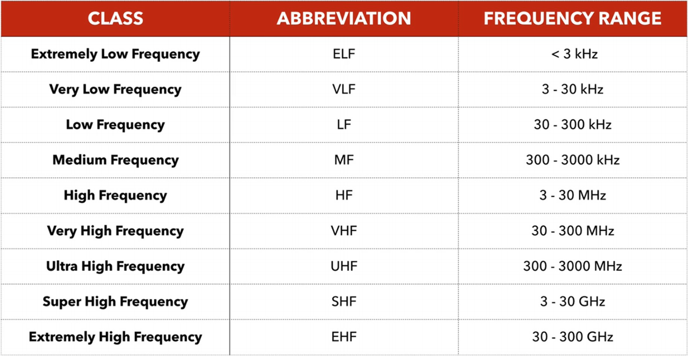
Different frequency bands and their classification (Source: https://en.wikipedia.org/wiki/Radio_spectrum )
RTL-SDR: 52-2200 MHz
HackRF: 1 MHz to 6 GHz
Yardstick one: Sub 1 GHz
LimeSDR: 100 kHz to 3.8 GHz
To give you a perspective of the frequencies just mentioned, a human ear can listen to a 20 Hz to 20 kHz frequency range. The Wi-Fi and BLE devices that you have operate at 2.4 GHz.
Antenna
An antenna is the component responsible for converting the information into electromagnetic signals that can travel through the medium of propagation (usually air). If you have noticed the metallic receivers that you adjusted for listening to FM or on old television sets, they are a good example of how an antenna might look like.
- 1.
Log periodic antennas.
- 2.
Traveling wave antennas.
- 3.
Microwave antennas.
- 4.
Reflector antennas.
- 5.
Wire antennas.
We won’t go into the specifics of each antenna, as the choice of an antenna is highly dependent on the specific usage. However, if you are interested, you can learn more about antennas at https://www.tutorialspoint.com/antenna_theory/antenna_theory_quick_guide.htm .
Gain
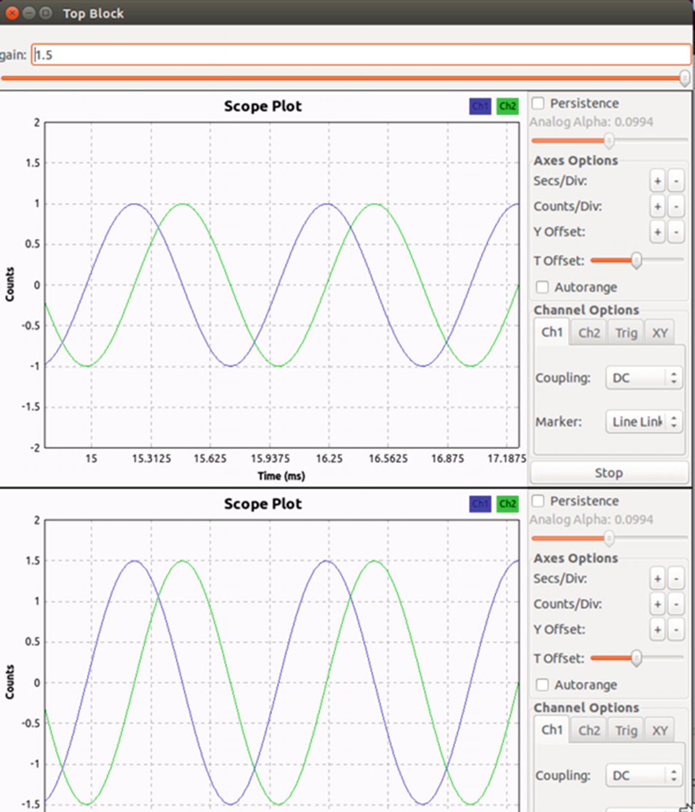
Comparison between an original signal and a signal with 1.5 gain
The top waveform in Figure 9-6 is the original signal whereas the bottom one has a gain of 1.5. As you can see, the new output signal is 1.5 times that of the original input signal.
In most practical cases, you will see gain being used because the signal received from air is often very weak, which makes the processing difficult. The value of gain should be chosen carefully, as setting the gain to be extremely high would end up distorting the signal, making it unreadable.
Filters
Filters in radio communications are used for the same purpose as their name suggests. They help to filter out unnecessary data (or even sometimes the required data) from the overall signal.
- 1.
Low pass filter: Allows all frequencies lower than the threshold frequency.
- 2.
High pass filter: Allows all frequencies higher than the threshold frequency.
- 3.
Band pass filter: Allows all frequencies within the band frequency range.
You will find yourself using filters in a number of situations when you have to perform activities such as eliminating noisy signals or separating one signal from the others.
GNURadio for Radio Signal Processing
GNURadio is an open source SDK to handle digital and analog signal processing. It also supports a wide range of SDR hardware tools such as RTL-SDR, HackRF, USRP, and more, and includes a huge variety of radio processing blocks and applications that can be used to process the data.
It serves a number of purposes for security research, including things such as analyzing a captured signal, performing demodulation, extracting data from signals, reversing unknown protocols, and more. It is also used to perform audio processing, mobile communication analysis, flight and satellite tracking, RADAR systems, and more advanced signal processing applications.
GNURadio, simply put, is an open source tool that allows you to work with various radio components. You can have various input sources, processing blocks, and output forms. GNURadio applications can also be built using Python scripting, which internally call the C++ signal processing code of GNURadio and give the desired output. GNURadio Companion is a graphical utility that comes along with the GNURadio toolkit that allows you to build flow graphs using the underlying GNURadio components.
Working with GNURadio
To understand GNURadio, we start with a very simple flow graph. In our first exercise, we generate a sinusoidal wave and send it to a Transmission Control Protocol (TCP) sink. In another program, we use a TCP source, pointing it to the input signal coming from the previous program and then finally plot the entire waveform. We learn more about the components as we encounter them further in the exercises.
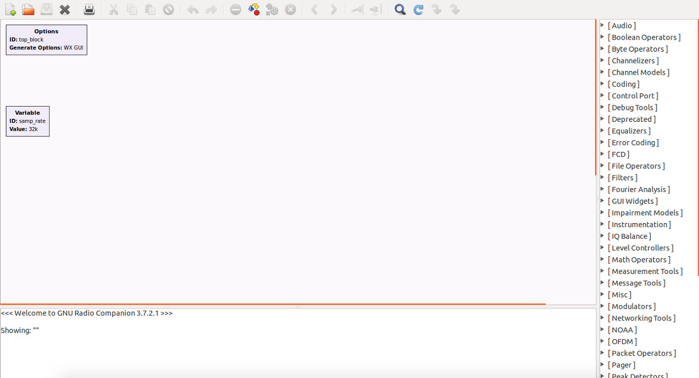
GNURadio workspace
Workspace: The blank area with two blocks named Options and Variable.
Blocks: The right-side list of all the various processing blocks you can use to build your radio.
Reports: The bottom pane of the screen that shows output, debug, and error messages.
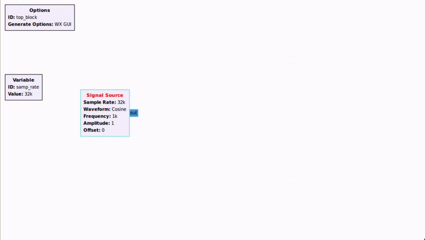
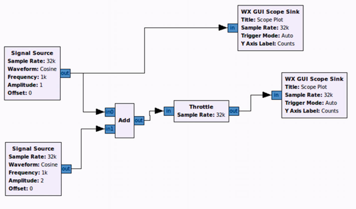
Adding a signal source
As you can see, we now have the Signal Source block in our Workspace. Notice that the color of the Signal Source text is red because we have not yet connected the output coming out of the block (in this case a cosine waveform coming out of the signal source) to another block.
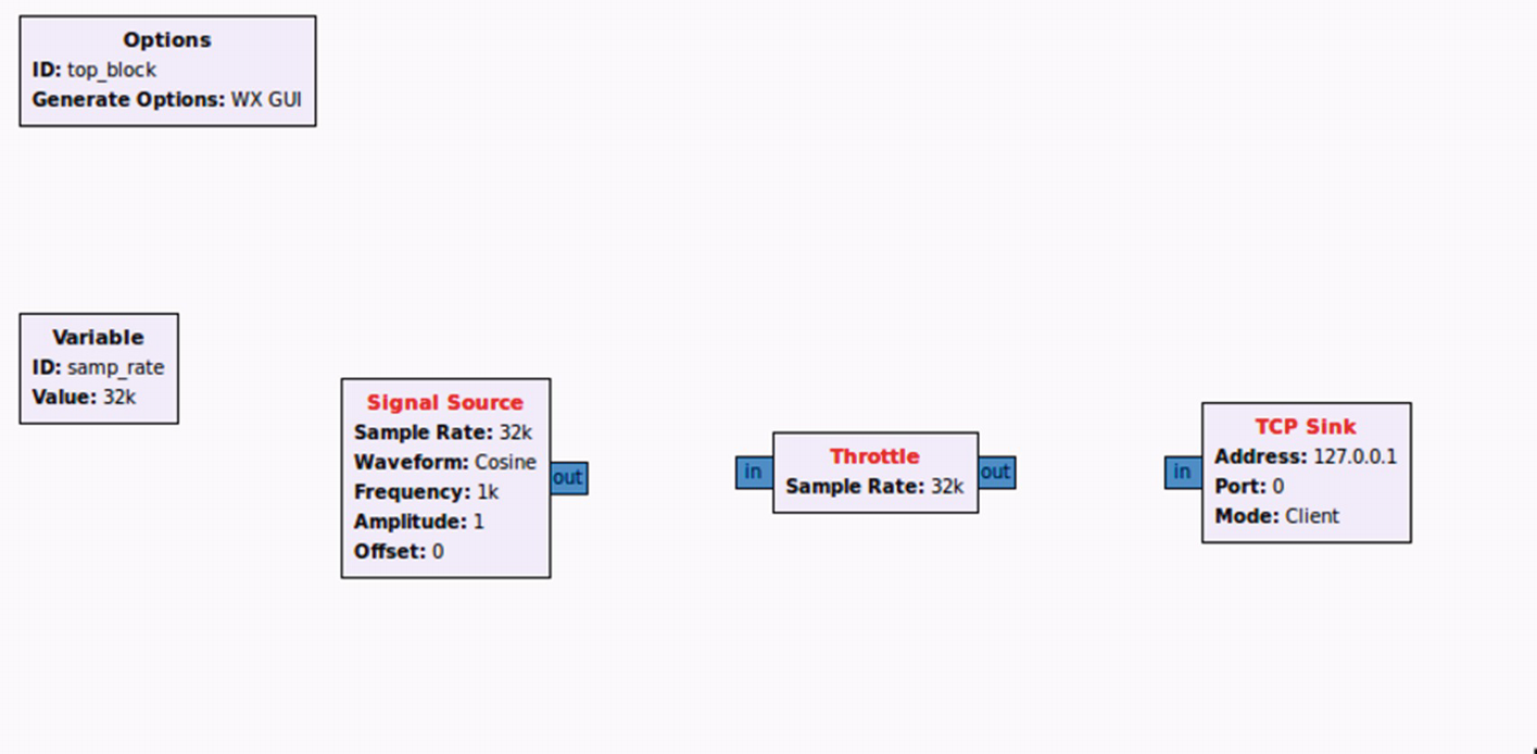
All blocks added
The next step would be to connect the blocks to each other. This can be done by clicking the Out tab of one block and the In tab of the other block we want to connect. Once done, double-click TCP Sink, which should open up the block’s properties.
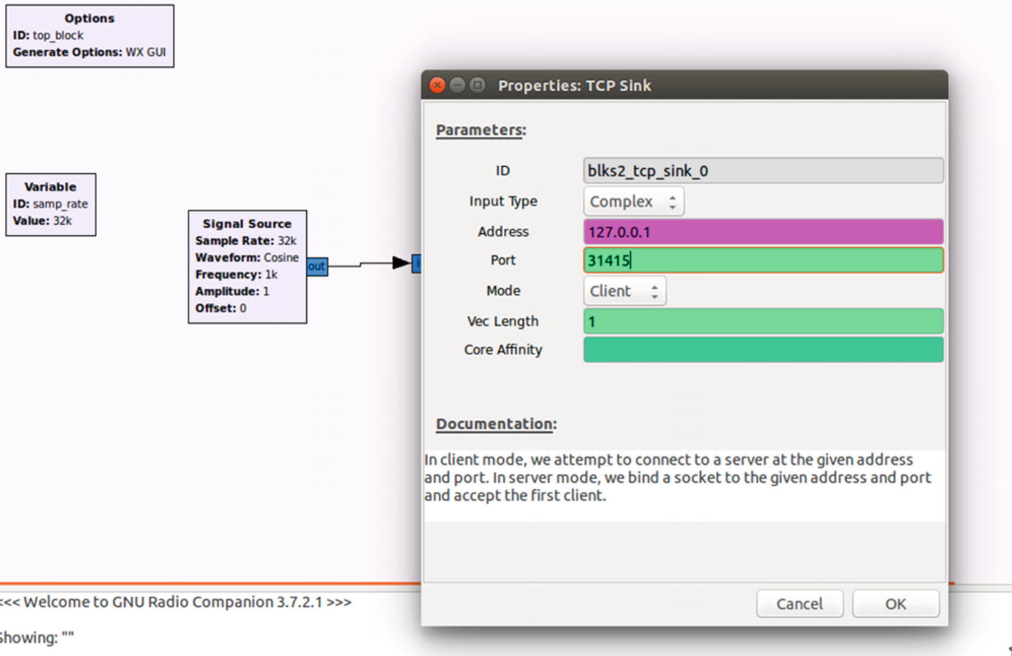
Modifying properties
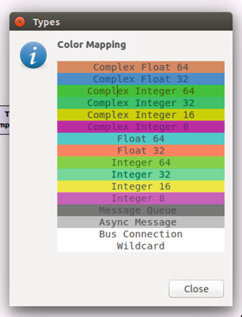
Data types color mapping
Returning to our flow graph, the next thing that we need to do is create another GNURadio companion (.grc) file that would take the input coming from our first program and plot it for us.
To do this, simply save the existing flow graph and create a new file in GNURadio. In the new file, drag and drop TCP Source, Throttle, and Scope Sink. Edit the property of the TCP Source block’s Port value to 31415.
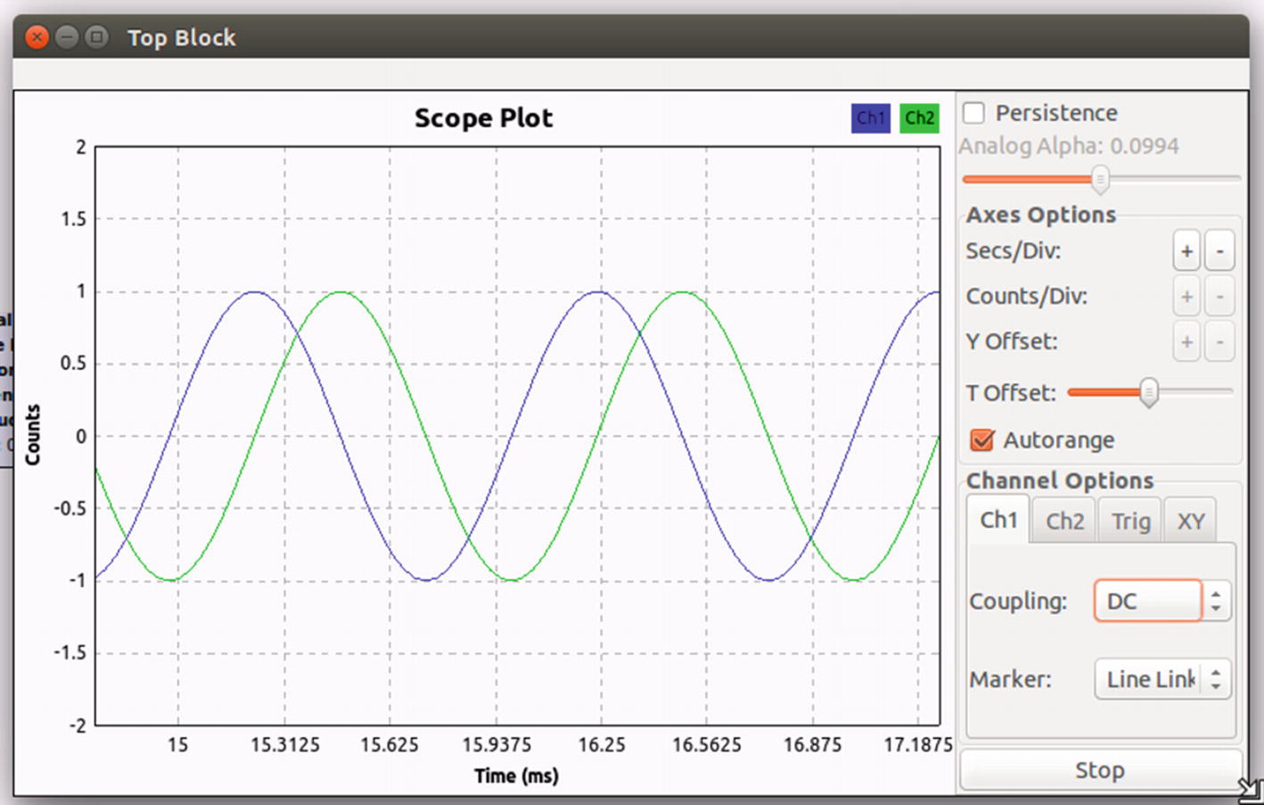
Plotted waveform
As you can see, we just created our radio, starting with a signal generator block, and sent it to a TCP sink, which was received by the TCP source in the other program, and finally created a waveform plot with it.
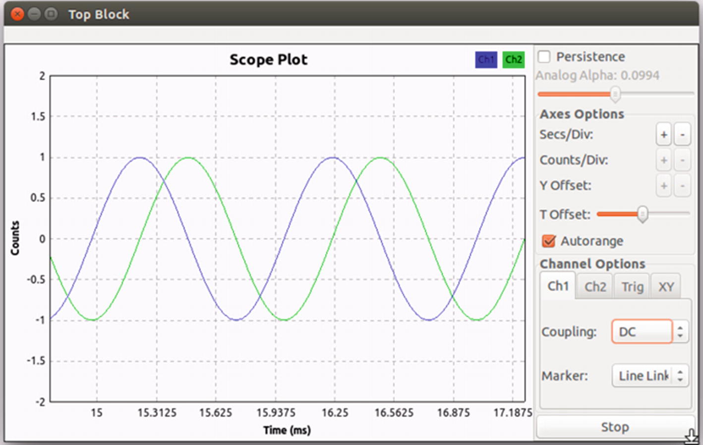
Initial waveform
Final workspace
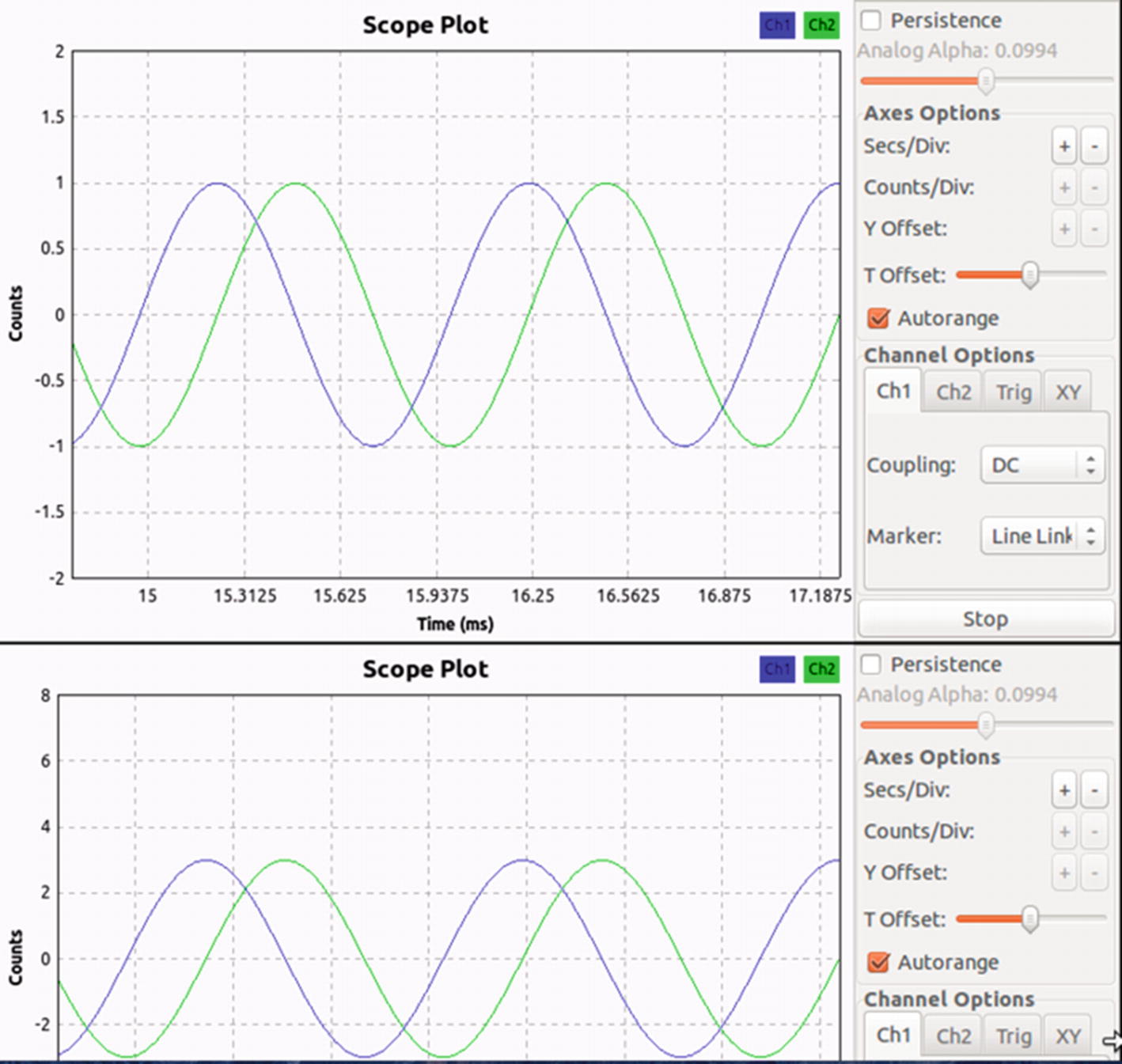
Analyzing changes between two different waveforms
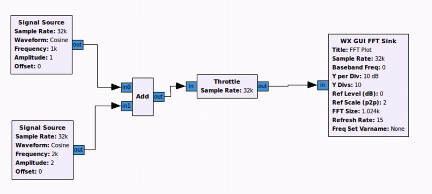
Understanding FFT workspace
Fast Fourier transform
Identifying the Frequency of a Target
One of the most important pieces of analysis that we have to do when we start any IoT device radio analysis is to identify its operating frequency. This information can sometimes be publicly available via the FCC ID information or on the device’s web site or community forums.
If it is not present and not easily obtainable, we can use our own tools and techniques to find out which frequency (or frequency range) the device is active on. For this, we use an SDR tool such as RTL-SDR, which will allow us to monitor a wide range of frequency spectrums covering the frequency on which the device would most often be operating. The software utility that we use to look at the frequency spectrum is GQRX.
- 1.
Garage door opener key fob.
- 2.
Weather station.
- 1.
Garage door opener key fob: It’s an inexpensive (< $10) piece of hardware without any visible FCC ID or any other kind of certification marked on the device. If we open up the key fob as shown in Figure 9-18, we see that it uses a 433 MHz oscillator.

Opening a key fob for analysis
- 2.
Weather station: In comparison to key fob, we are a bit lucky in this case, as this weather thermometer has a clearly marked FCC ID on the back of the device, as shown in Figure 9-19.
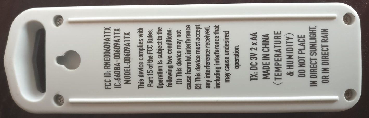
Weather station with clear FCC ID on the back
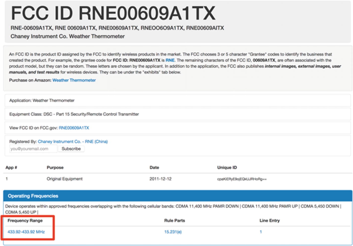
Weather thermometer FCC ID information
Now that we have identified the frequency of both our devices, we can use the tool GQRX to confirm our findings and identify the exact frequencies up to three to four decimal places on which these devices are operating. GQRX is a tool based on GNURadio and the QT framework to provide us with a visual analysis of the entire frequency spectrum. There are a lot of other use cases and modifications you can do with GQRX, but I won’t go into that here. If you are interested, you can find more information on the official web site at http://gqrx.dk/category/doc .

Analyzing exact frequency of target device using GQRX
Once you start the devices, you will begin noticing the peaks (or spikes) in the frequency spectrum shown in the top window pane. You will also notice the values creating an impact in the lower pane of the window, which is known as the waterfall view. In our case, the peak is close to 433.897 and the exact frequency we have here is 433.92 MHz.
Analyzing the Data
Now that we have identified the exact frequencies which the devices operate on using GQRX, the next step for us would be to figure out exactly what data are being transmitted through the devices, and if required, decode them into a readable format. Given the fact that both of these devices operate on the 433 MHz frequency, we can use a utility provided along with the RTL-SDR tools called rtl_433 to analyze the data.
Analyzing Using RTL_433 and Replay
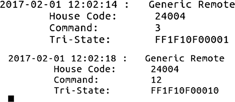
Key fob data
We can also notice here that for each key fob press, the hex value being transmitted changes a bit.
From here on, you can either use a tool like HackRF to transmit the packets again, or even a combination of Arduino and 433 MHz transmitter would work. Let’s go ahead and have a look at how this could be done using Arduino and a 433 MHz transmitter.
Arduino 5V ⇐> VCC of both transmitter and receiver.
Arduino GND ⇐> GND of both transmitter and receiver.
Arduino D10 ⇐> Data of transmitter.
Arduino D2 ⇐> Data of receiver.
Next, download the Arduino library for the RC_Switch, which contains the program for transmitting data on 433 MHz, from https://github.com/sui77/rc-switch .
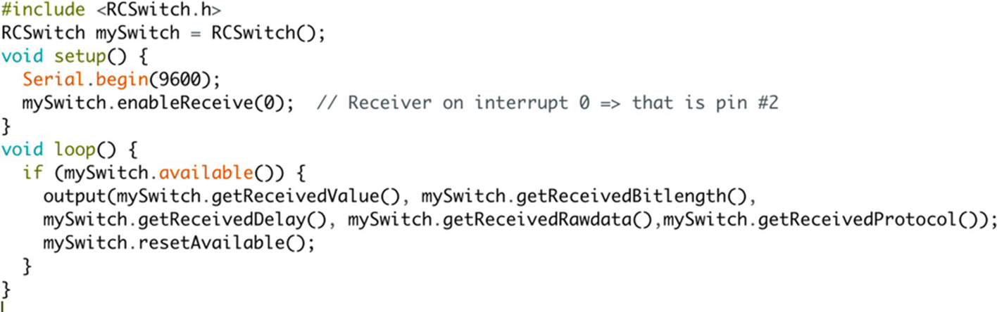
ReceiveAdvanced code
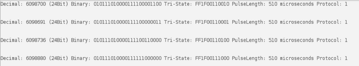
Showing the decoded data of a key fob with different key presses

SendDemo code
Once you run the SendDemo code, you will be able to replay the radio packets, making the garage door open. Notice that we are looking at a case where there is no verification of existing code being reused to open the garage door. In other cases, though, you will need to perform additional steps to ensure that the replay attack works, which can be made by jamming the signal and capturing so that we have an unused radio packet with us that can be used by us.
Using GNURadio to Decode Data
Now that we know how to replay data by first sniffing RTL-SDR and sending using the Arduino and 433 MHz setup, we can move on to decoding the data of the weather station. Unlike the garage door opener key fob, the weather station transmits data that are not easily understandable. Therefore, we will need to use the GNURadio and its radio processing blocks to be able to figure out exactly what data are being sent by sniffing the packets.
Once you start analyzing the GQRX or GNURadio analysis of the frequency on which the weather station operates, you will be able to see various peaks and bursts of data that are sent at regular intervals. Here we are trying to figure out what the exact data are that are being sent by the weather station.
Let’s go ahead and create a GNURadio workflow to decode the data that are being transmitted by the weather station.
First, open a GNURadio companion and set the Generate Options to WX. Change the sample rate to 1M.
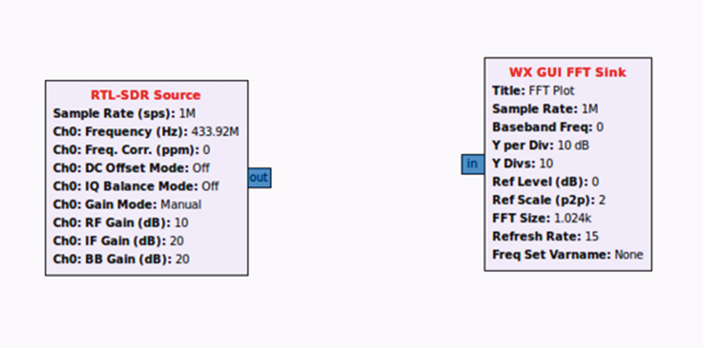
Initial flow graph
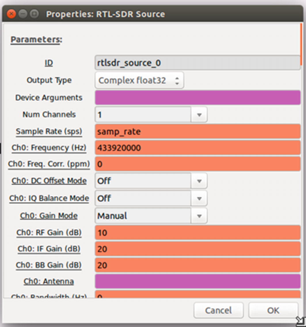
Setting RTL-SDR block properties in GNURadio
For this reason, we will have to use an additional block of Complex to Mag ^ 2 to convert this to a usable positive value. Drag and drop a Complex to Mag^2 block to the workflow and connect the output of the RTL-SDR source to Complex to Mag^2.
Because the signal at this stage might be a bit weak, it’s a good idea to amplify the signal by adding a Multiply Const block. We can set the constant value to be 20, which is a suitable amplification value.
Wav File Sink : This will save the output result to a .wav file that we can then analyze in a tool such as Audacity. Double-click this block and put it in a location where you would like to save the output file.
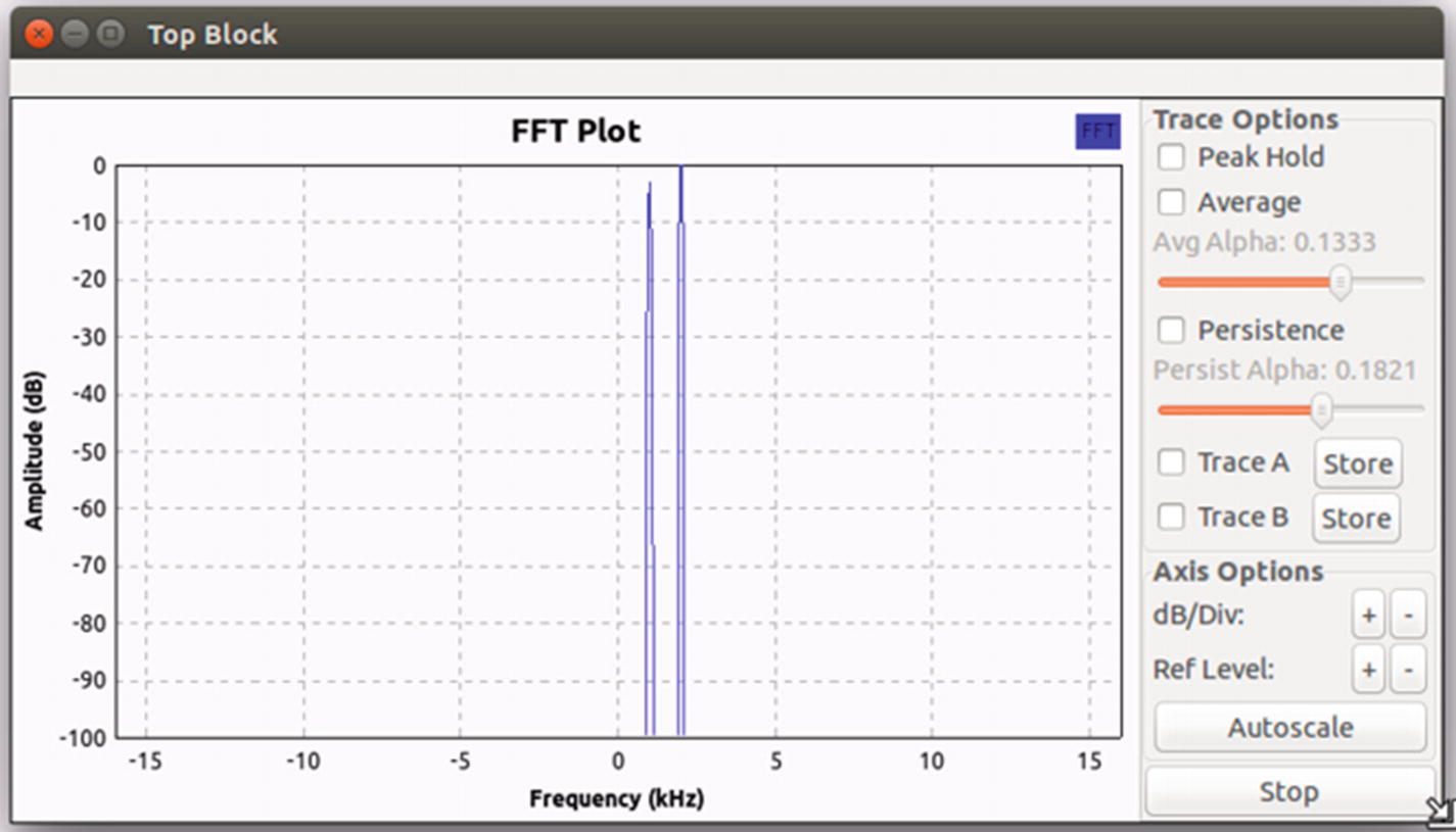
WX GUI FFT Sink : This is added for us to see the output as a waveform plot in the frequency domain.
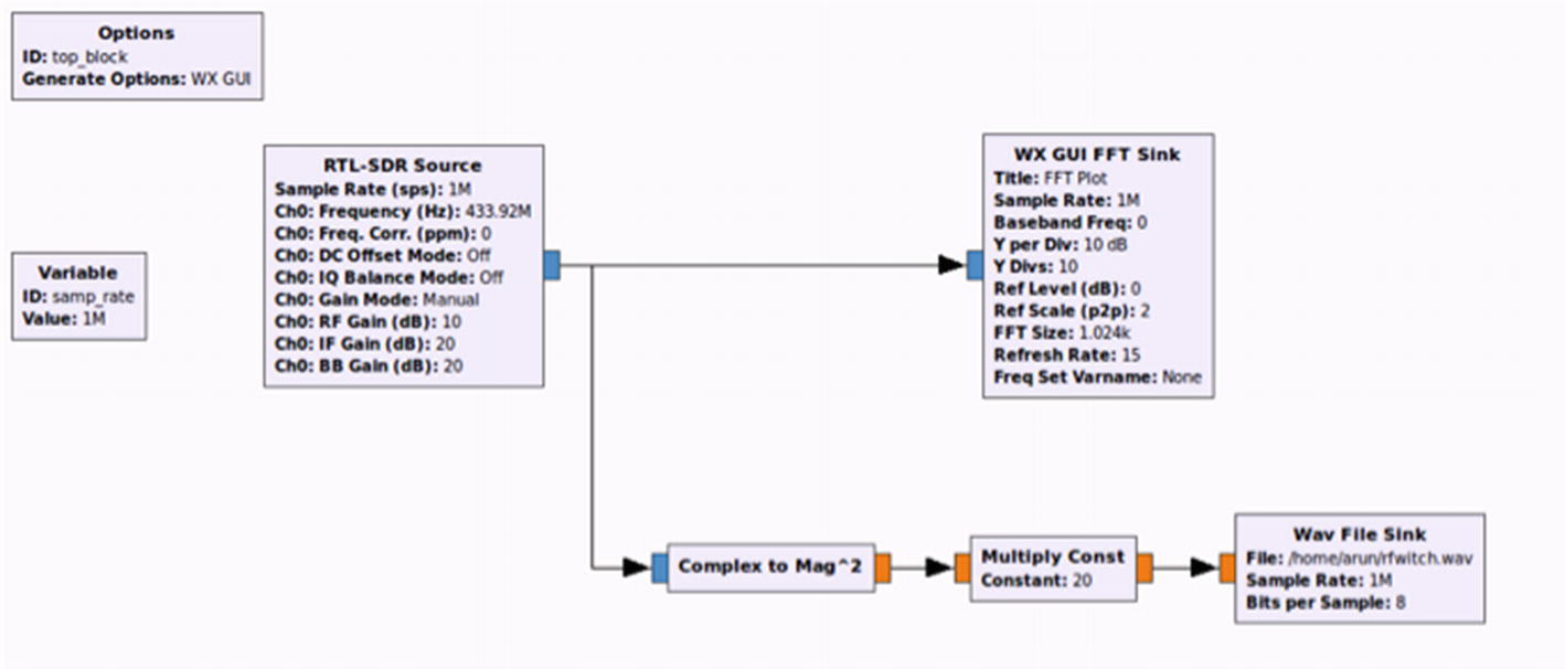
Final GNURadio flow graph

FFT plot of the signal
Let’s go ahead and now open the .wav file created in Audacity. Audacity is a tool for audio analysis and editing, but it can also be used to analyze radio signals as in our example.
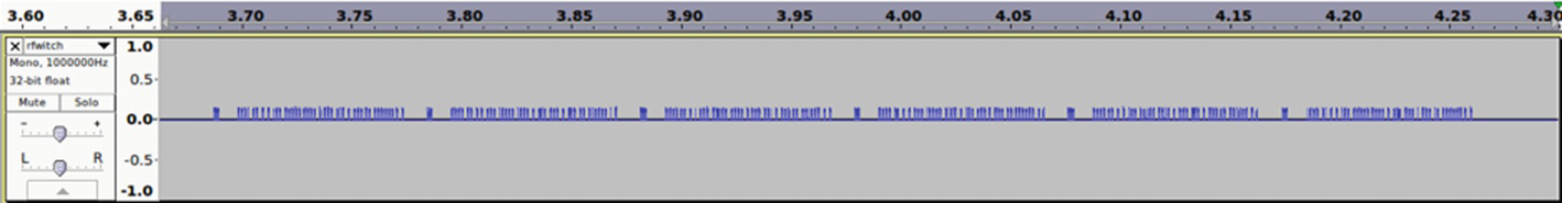
Waveform display before Multiply Const
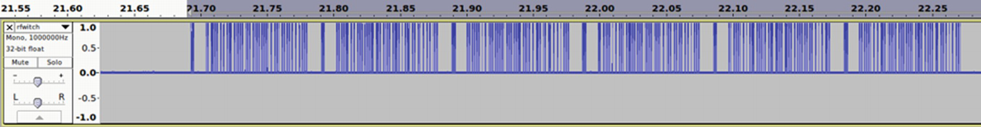
Waveform display after Multiply Const
As we can see from Figure 9-31, it looks like an on-off keying (OOK), which is a form of amplitude-shift keying (ASK) modulation. The shorter pulse represents a digital 0 and a longer pulse represents a digital 1.
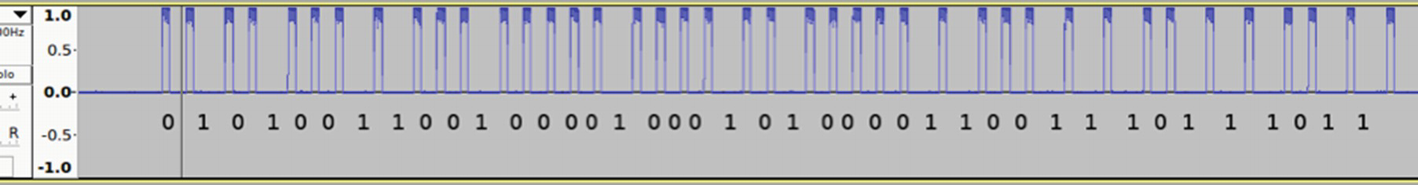
Analyzing the output .wav file and calculating 1s and 0s
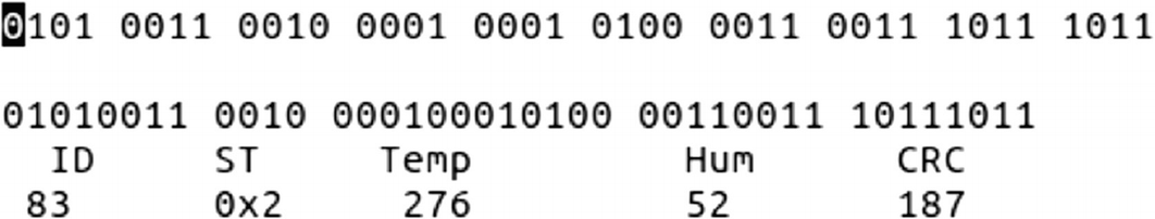
Final decoded data
That is how we can identify, analyze, and decode data using tools such as RTL-SDR, GNURadio, and GQRX.
Replaying Radio Packets
One of the other important concepts in working with radios is the ability to replay data. Even though we had a look at replaying using a 433 MHz transmitter, this might not always apply when you encounter a device on a less popular frequency. If the frequency that you are working with is somewhat less popular, you might not be able to find the transmitting module that easily. In those cases, a device like HackRF is invaluable.
HackRF is an open source device developed by Michael Ossman (with contributions from numerous contributors, including Jared Boone and Dominic Spill) to analyze and assess radio frequencies in a wide range from 1 MHz to 6 GHz. Because we have already installed the HackRF tools, we can now go ahead and start using them.
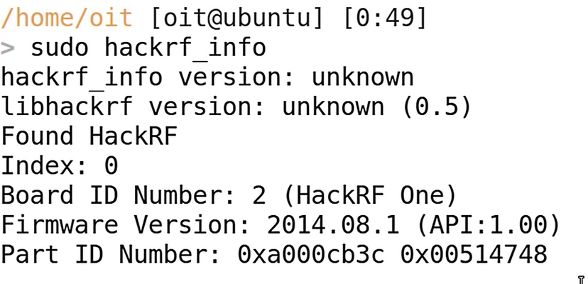
HackRF device connected to the system
Once we have verified that the HackRF device is connected and accessible, the next step is to use hackrf_transfer to store the packet captures in a file that we can later use to replay. We also use additional parameters such as –r to specify the read file where captured packets will be stored, -f for the frequency that we want to work with, and –s for the sample rate.

Capturing packets with HackRF
Once you have captured the packets, the next step is to simply replay them, which can be done by simply replacing the –r with –t, to specify the file name from which transmit data will be taken.
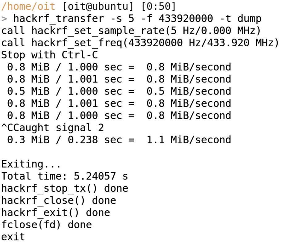
Replaying packets with HackRF
Conclusion
We went through a number of concepts in this chapter, including how to get started with SDR, as well as a firsthand experience working with radio signals and decoding the data.
We also gained familiarity with tools such as RTL-SDR, GQRX, GNURadio, and HackRF. These concepts, even though covered briefly in this chapter, will be useful in a lot of practical situation. I have used GNURadio in most of my IoT pentesting engagements where I have to decode radio communication being performed, or to reverse engineer an unknown protocol.
I strongly recommended that you try out these topics by yourself on real-world devices and real-world packet captures.