
Multiplying Matrices
Multiplication is the tool you’ll use to perform transformations like scaling, rotation, and translation. It’s certainly possible to apply them one at a time, sequentially, but in practice you’ll often want to apply several transformations at once. Multiplying them together is how you make that happen, as you’ll see when you get to Chapter 4, Matrix Transformations.
So let’s talk about matrix multiplication. It takes two matrices and produces another matrix by multiplying their component elements together in a specific way. You’ll see how that works shortly, but start first by writing a test that describes what you expect to happen when you multiply two 4x4 matrices together. Don’t worry about 2x2 or 3x3 matrices here; your ray tracer won’t need to multiply those at all.
| | Scenario: Multiplying two matrices |
| | Given the following matrix A: |
| | | 1 | 2 | 3 | 4 | |
| | | 5 | 6 | 7 | 8 | |
| | | 9 | 8 | 7 | 6 | |
| | | 5 | 4 | 3 | 2 | |
| | And the following matrix B: |
| | | -2 | 1 | 2 | 3 | |
| | | 3 | 2 | 1 | -1 | |
| | | 4 | 3 | 6 | 5 | |
| | | 1 | 2 | 7 | 8 | |
| | Then A * B is the following 4x4 matrix: |
| | | 20| 22 | 50 | 48 | |
| | | 44| 54 | 114 | 108 | |
| | | 40| 58 | 110 | 102 | |
| | | 16| 26 | 46 | 42 | |
Let’s look at how this is done for a single element of a matrix, going step-by-step to find the product for element C10, highlighted in the figure.
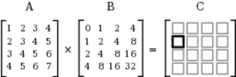
Element C10 is in row 1, column 0, so you need to look at row 1 of the A matrix, and column 0 of the B matrix, as shown in the following figure.
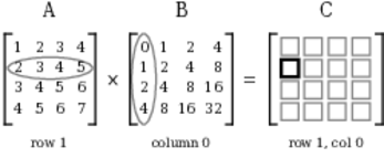
Then, you multiply corresponding pairs of elements together (A10 and B00, A11 and B10, A12 and B20, and A13 and B30), and add the products. The following figure shows how this comes together.

The result, here, is 31, and to find the other elements, you perform this same process for each row-column combination of the two matrices.
Stated as an algorithm, the multiplication of two 4x4 matrices looks like this:
- Let A and B be the matrices to be multiplied, and let M be the result.
- For every row r in A, and every column c in B:
- Let Mrc = Ar0 * B0c + Ar1 * B1c + Ar2 * B2c + Ar3 * B3c
As pseudocode, the algorithm might look like this:
| | function matrix_multiply(A, B) |
| | M ← matrix() |
| | |
| | for row ← 0 to 3 |
| | for col ← 0 to 3 |
| | M[row, col] ← A[row, 0] * B[0, col] + |
| | A[row, 1] * B[1, col] + |
| | A[row, 2] * B[2, col] + |
| | A[row, 3] * B[3, col] |
| | end for |
| | end for |
| | |
| | return M |
| | end function |
If this all feels kind of familiar, it might be because you’ve already implemented something very similar—the dot product of two vectors. Yes, it’s true. Matrix multiplication computes the dot product of every row-column combination in the two matrices! Pretty cool.
Now, we’re not done yet. Matrices can actually be multiplied by tuples, in addition to other matrices. Multiplying a matrix by a tuple produces another tuple. Start with a test again, like the following, to express what you expect to happen when multiplying a matrix and a tuple.
| | Scenario: A matrix multiplied by a tuple |
| | Given the following matrix A: |
| | | 1 | 2 | 3 | 4 | |
| | | 2 | 4 | 4 | 2 | |
| | | 8 | 6 | 4 | 1 | |
| | | 0 | 0 | 0 | 1 | |
| | And b ← tuple(1, 2, 3, 1) |
| | Then A * b = tuple(18, 24, 33, 1) |
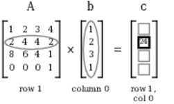
How does it work? The trick begins by treating the tuple as a really skinny (one column!) matrix, like this:
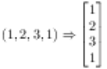
Four rows. One column.
It comes together just as it did when multiplying two 4x4 matrices together, but now you’re only dealing with a single column in the second “matrix.” The following figure illustrates this, highlighting the row and column used when computing the value of c10.
To compute the value of c10, you consider only row 1 of matrix A, and column 0 (the only column!) of tuple b. If you think of that row of the matrix as a tuple, then the answer is found by taking the dot product of that row and the other tuple:
The other elements of c are computed similarly. It really is the exact same algorithm used for multiplying two matrices, with the sole difference being the number of columns in the second “matrix.”
|
|
If you’re feeling uncomfortable with how much magic there is in these algorithms, check out “An Intuitive Guide to Linear Algebra”[12] on BetterExplained.com. It does a good job of making sense of this stuff! |
Pause here to make the tests pass that you’ve written so far. Once you have them working, carry on! We’re going to look at a very special matrix, and we’ll use multiplication to understand some of what makes it so special.