
Surface Normals
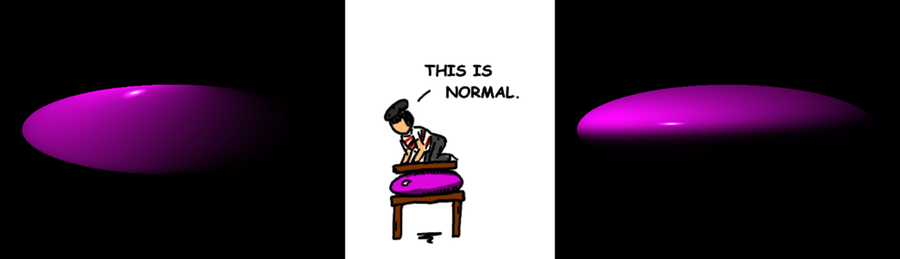
A surface normal (or just normal) is a vector that points perpendicular to a surface at a given point. Consider a table, as shown in the following figure.
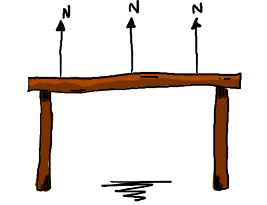
A flat surface like a table will have the same normal at every point on its surface, as shown by the vectors labeled N. If the table is level, the normals will be the same as “up,” but even if we tilt the table, they’ll still be perpendicular to the table’s surface, like the following figure shows.

Things get a little trickier when we start talking about nonplanar surfaces (those that aren’t uniformly flat). Take the planetoid in the following figure for example.

The three normal vectors certainly aren’t all pointing the same direction! But each is perpendicular to the surface of the sphere at the point where it lives.
Let’s look at how to actually compute those normal vectors.
Computing the Normal on a Sphere
Start by writing the following tests to demonstrate computing the normal at various points on a sphere. Introduce a new function, normal_at(sphere, point), which will return the normal on the given sphere, at the given point. You may assume that the point will always be on the surface of the sphere.
| | Scenario: The normal on a sphere at a point on the x axis |
| | Given s ← sphere() |
| | When n ← normal_at(s, point(1, 0, 0)) |
| | Then n = vector(1, 0, 0) |
| | |
| | Scenario: The normal on a sphere at a point on the y axis |
| | Given s ← sphere() |
| | When n ← normal_at(s, point(0, 1, 0)) |
| | Then n = vector(0, 1, 0) |
| | |
| | Scenario: The normal on a sphere at a point on the z axis |
| | Given s ← sphere() |
| | When n ← normal_at(s, point(0, 0, 1)) |
| | Then n = vector(0, 0, 1) |
| | |
| | Scenario: The normal on a sphere at a nonaxial point |
| | Given s ← sphere() |
| | When n ← normal_at(s, point(√3/3, √3/3, √3/3)) |
| | Then n = vector(√3/3, √3/3, √3/3) |
One other feature of these normal vectors is hiding in plain sight: they’re normalized. Add the following test to your suite, which shows that a surface normal should always be normalized.
| | Scenario: The normal is a normalized vector |
| | Given s ← sphere() |
| | When n ← normal_at(s, point(√3/3, √3/3, √3/3)) |
| | Then n = normalize(n) |
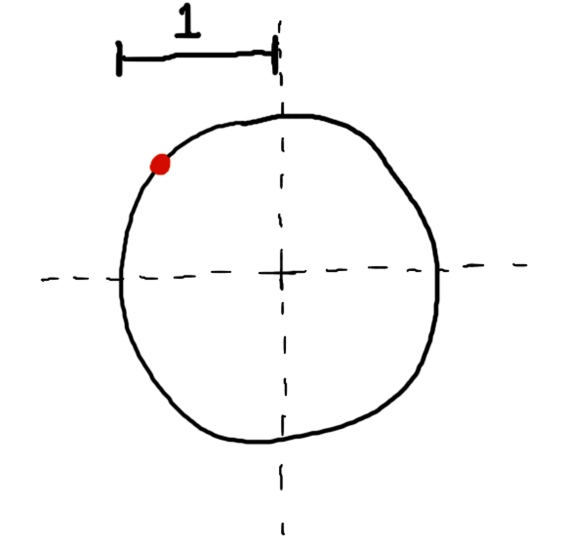
Now, let’s make those tests pass by implementing that normal_at function. To understand how it will work its magic, take a look at the unit circle in the following figure. It’s centered on the origin, and a point (presumably a point of intersection) has been highlighted on its circumference.
Let’s say you want to find the normal at that highlighted point. Draw an arrow from the origin of the circle to that point, as in the following figure.
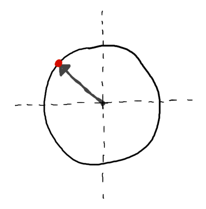
It turns out that this arrow—this vector!—is perpendicular to the surface of the circle at the point where it intersects. It’s the normal! Algorithmically speaking, you find the normal by taking the point in question and subtracting the origin of the sphere ((0,0,0) in your case). Here it is in pseudocode:
| | function normal_at(sphere, p) |
| | return normalize(p - point(0, 0, 0)) |
| | end function |
(Note that, because this is a unit sphere, the vector will be normalized by default for any point on its surface, so it’s not strictly necessary to explicitly normalize it here.)
If only that were all there were to it! Sadly, the sphere’s transformation matrix is going to throw a (small) wrench into how the normal is computed. Let’s take a look at what needs to happen for the normal calculation to compensate for a transformation matrix.
Transforming Normals
Imagine you have a sphere that has been translated some distance from the world origin. If you were to naively apply the algorithm above to find the normal at almost any point on that sphere, you’d find that it no longer works correctly. The figure shows how it goes wrong in this case. On the left, the normal for a sphere at the origin is computed. On the right, the normal is computed for a sphere that has been moved away from the origin.
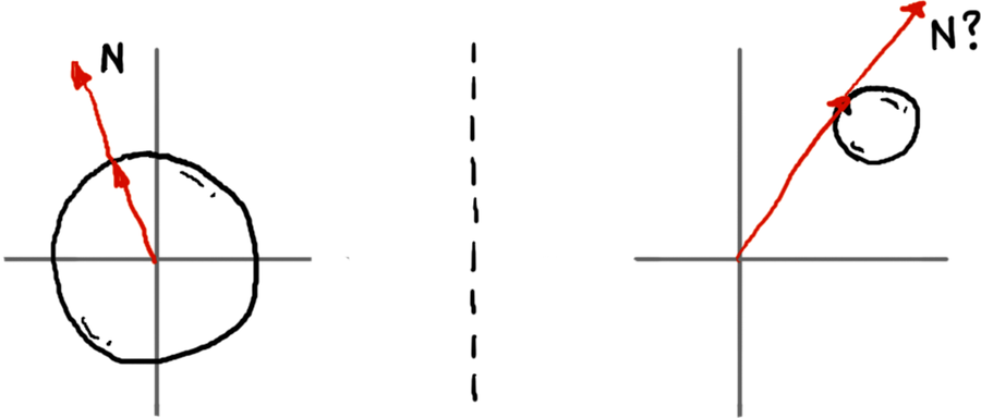
The “normal” on the right is not remotely normalized, and is not even pointing in the correct direction. Why? The problem is that your most basic assumption has been broken: the sphere’s origin is no longer at the world origin.
Write the following tests to show what ought to happen. They demonstrate computing the normal first on a translated sphere and then on a scaled and rotated sphere.
| | Scenario: Computing the normal on a translated sphere |
| | Given s ← sphere() |
| | And set_transform(s, translation(0, 1, 0)) |
| | When n ← normal_at(s, point(0, 1.70711, -0.70711)) |
| | Then n = vector(0, 0.70711, -0.70711) |
| | |
| | Scenario: Computing the normal on a transformed sphere |
| | Given s ← sphere() |
| | And m ← scaling(1, 0.5, 1) * rotation_z(π/5) |
| | And set_transform(s, m) |
| | When n ← normal_at(s, point(0, √2/2, -√2/2)) |
| | Then n = vector(0, 0.97014, -0.24254) |
These won’t pass yet, but you’ll turn them green in just a moment.
Remember back when we talked about World Space vs. Object Space? It turns out that this distinction between world and object space is part of the solution to this conundrum, too. You have a point in world space, and you want to know the normal on the corresponding surface in object space. What to do? Well, first you have to convert the point from world space to object space by multiplying the point by the inverse of the transformation matrix, thus:
| | object_point ← inverse(transform) * world_point |
With that point now in object space, you can compute the normal as before, because in object space, the sphere’s origin is at the world’s origin. However! The normal vector you get will also be in object space…and to draw anything useful with it you’re going to need to convert it back to world space somehow.
Now, if the normal were a point you could transform it by multiplying it by the transformation matrix. After all, that’s what the transformation matrix does: it transforms points from object space to world space. And in truth, this almost works here, too. Consider the following two images of a squashed sphere, which has been scaled smaller in y. The normal vectors of the one on the left have been multiplied by the transformation matrix. The one on the right is how the sphere is supposed to look.
The one on the left definitely looks…off. It’s as if someone took a picture of a regular, untransformed sphere, and squashed that, rather than squashing the sphere itself. What’s the difference?
It all comes down to how the normal vectors are being transformed. The following illustration shows what happens. The sphere is scaled in y, squashing it vertically, and the normals are multiplied by the transformation matrix.
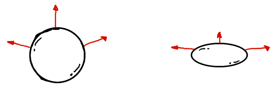
As you can see, multiplying by the transformation matrix doesn’t preserve one of the fundamental properties of normal vectors in this case: the normal is not necessarily going to be perpendicular to the surface after being transformed!
So how do you go about keeping the normals perpendicular to their surface? The answer is to multiply the normal by the inverse transpose matrix instead. So you take your transformation matrix, invert it, and then transpose the result. This is what you need to multiply the normal by.
| | world_normal ← transpose(inverse(transform)) * object_normal |
Be aware of two additional things here:
- Technically, you should be finding submatrix(transform, 3, 3) (from Spotting Submatrices) first, and multiplying by the inverse and transpose of that. Otherwise, if your transform includes any kind of translation, then multiplying by its transpose will wind up mucking with the w coordinate in your vector, which will wreak all kinds of havoc in later computations. But if you don’t mind a bit of a hack, you can avoid all that by just setting world_normal.w to 0 after multiplying by the 4x4 inverse transpose matrix.
- The inverse transpose matrix may change the length of your vector, so if you feed it a vector of length 1 (a normalized vector), you may not get a normalized vector out! It’s best to be safe, and always normalize the result.
In pseudocode, then, your normal_at function should look something like the following.
| | function normal_at(sphere, world_point) |
| | object_point ← inverse(sphere.transform) * world_point |
| | object_normal ← object_point - point(0, 0, 0) |
| | world_normal ← transpose(inverse(sphere.transform)) * object_normal |
| | world_normal.w ← 0 |
| | return normalize(world_normal) |
| | end function |
Go ahead and pause here while you get things working to this point. Once your tests are all green, let’s talk about how to compute the reflection vector.