
Cones
Okay. Next you’re going to add cones to your ray tracer, and it turns out that cones are remarkably similar to cylinders. A true cone has these features:
- It is infinite in length, just like a cylinder.
- It can be truncated, just like a cylinder.
- It can be closed, just like a cylinder.
And I really do mean just like a cylinder. You may be able to reuse a fair bit of the code you just wrote for cylinders.
Here’s where the challenge ramps up, though—I’m going to take the training wheels off. No hand-holding. No safety nets. Just a bit of explanation, a few tests, and a whole heap of confidence in your ability to do just about anything you put your mind to.
You’re going to implement what is called a double-napped cone, which most folks would actually call two cones: one upside down, the other right-side up, with their tips meeting at the origin and extending toward infinity in both directions, as depicted in the following figure.

To render this, you’ll need to implement its intersection algorithm and the algorithm to compute its normal vector.
The intersection algorithm works almost exactly like the cylinder’s, but a, b, and c are computed differently. Given a ray’s origin o and direction vector d, the following formulas replace the ones you used for cylinders:
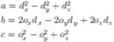
When a is zero, it means the ray is parallel to one of the cone’s halves, like so:

As you can see, this still means the ray might intersect the other half of the cone. In this case the ray will miss when both a and b are zero. If a is zero but b isn’t, you’ll use the following formula to find the single point of intersection:
If a is nonzero, you’ll use the same algorithm, but with the new a, b, and c, that you used for the cylinders.
Here are two tests to help you double-check your cone intersections:
| | Scenario Outline: Intersecting a cone with a ray |
| | Given shape ← cone() |
| | And direction ← normalize(<direction>) |
| | And r ← ray(<origin>, direction) |
| | When xs ← local_intersect(shape, r) |
| | Then xs.count = 2 |
| | And xs[0].t = <t0> |
| | And xs[1].t = <t1> |
| | |
| | Examples: |
| | | origin | direction | t0 | t1 | |
| | | point(0, 0, -5) | vector(0, 0, 1) | 5 | 5 | |
| | | point(0, 0, -5) | vector(1, 1, 1) | 8.66025 | 8.66025 | |
| | | point(1, 1, -5) | vector(-0.5, -1, 1) | 4.55006 | 49.44994 | |
| | Scenario: Intersecting a cone with a ray parallel to one of its halves |
| | Given shape ← cone() |
| | And direction ← normalize(vector(0, 1, 1)) |
| | And r ← ray(point(0, 0, -1), direction) |
| | When xs ← local_intersect(shape, r) |
| | Then xs.count = 1 |
| | And xs[0].t = 0.35355 |
You’ll implement end caps for cones much as you did for cylinders, but with one difference: whereas cylinders have the same radius everywhere, the radius of a cone will change with y. In fact, a cone’s radius at any given y will be the absolute value of that y. This means the check_cap function will need to be adjusted to accept the y coordinate of the plane being tested (cone.minimum or cone.maximum, respectively) and treat that as the radius within which the point must lie.
Here’s a test for the cone end caps to help you with your implementation:
| | Scenario Outline: Intersecting a cone's end caps |
| | Given shape ← cone() |
| | And shape.minimum ← -0.5 |
| | And shape.maximum ← 0.5 |
| | And shape.closed ← true |
| | And direction ← normalize(<direction>) |
| | And r ← ray(<origin>, direction) |
| | When xs ← local_intersect(shape, r) |
| | Then xs.count = <count> |
| | |
| | Examples: |
| | | origin | direction | count | |
| | | point(0, 0, -5) | vector(0, 1, 0) | 0 | |
| | | point(0, 0, -0.25) | vector(0, 1, 1) | 2 | |
| | | point(0, 0, -0.25) | vector(0, 1, 0) | 4 | |
Lastly, for the normal vector, compute the end cap normals just as you did for the cylinder, but change the rest to the following, given in pseudocode:
| | y ← √(point.x² + point.z²) |
| | y ← -y if point.y > 0 |
| | |
| | return vector(point.x, y, point.z) |
Again, here’s a test to help you out:
| | Scenario Outline: Computing the normal vector on a cone |
| | Given shape ← cone() |
| | When n ← local_normal_at(shape, <point>) |
| | Then n = <normal> |
| | Examples: |
| | | point | normal | |
| | | point(0, 0, 0) | vector(0, 0, 0) | |
| | | point(1, 1, 1) | vector(1, -√2, 1) | |
| | | point(-1, -1, 0) | vector(-1, 1, 0) | |
As with the infinite cylinder, a double-napped cone is a bit unwieldy, but thanks to truncation, you can cut off any bits of those double cones that you don’t want. If you want a traditional unit cone, for example, you can truncate it at y=-1 and y=0, and then translate it up 1 unit in y.