
Appendix A. Campus Network Technologies
A campus network leverages several networking technologies to provide the required services of the network. Throughout this book a number of these technologies have been named and used within the campus network, varying from classic technologies like VLAN to new technological concepts like SDA. This appendix describes a conceptual overview of the technologies named and used throughout this book. The descriptions, although sometimes technical, are aimed to provide the reader with a conceptual understanding of the usage or workings of the technology. They are not a replacement for the technical documentation and technically oriented books available for studying and mastering new technologies.
The appendix is divided into groups of technologies and describes the following technologies:
Common Technologies
Intent-Based Networking within the campus network can be deployed using either in a Software-Defined Access (SDA) manner or in a classic VLAN (non-fabric) manner. Both types of deployments are good for Intent-Based Networking, where over time more campus networks will evolve to SDA (as that is the next generation of technologies suitable for campus networks). Both types of deployments leverage common technologies in the operation and configuration of the Intent-enabled campus network. The following paragraphs describe the concepts of these common technologies.
Network Plug and Play
Cisco Network Plug and Play (PnP) is a technology that is used to (automatically) provision new switches or routers in the network. The technology is available within DNA Center as well as Cisco APIC-EM. The technology is used for LAN Automation within Software Defined Access; it is also used for non-SDA deployments. Figure A-1 provides an overview of how Network PnP within Cisco APIC-EM is used to provision a device.

Figure A-1 Flow of Network PnP with Cisco APIC-EM
A field engineer racks and stacks the new network switch and attaches its uplinks to the distribution switch. In this case, the distribution switch is also the seed device.
Once the switch is started up, with an empty configuration, the Network PnP process is started in the background.
It is important not to touch anything on the console, as any character entered on the console results in aborting the PnP process.
The steps in this process are as follows:
Once booted, the new switch will perform a DHCP request using VLAN1 (untagged traffic as the switch doesn’t have knowledge on VLANs yet) or a specific PnP-VLAN learned via CDP.
The seed device provides an IP address to the new switch from a pool. This can be a local pool or a central DHCP server. In the DHCP response, DHCP Option 43 is used to provide information to the PnP agent about how to contact the provisioning server, Cisco APIC-EM in this example.
The new switch parses the DHCP response, and if it contains DHCP option 43, it will parse the text inside to extract the required details to connect to Cisco APIC-EM. The new switch will use its serial number to register it with Cisco APIC-EM using the protocol and port specified in the DHCP option. If there is no DHCP option 43 specified, the PnP agent on the new switch will try to use DNS to connect to pnpserver.customer.com and use the DNS name of pnpntpserver.customer.com for the NTP server. Customer.com is the domain suffix as specified in the DHCP scope.
Cisco APIC-EM registers the new device in the PnP application. Specific SSH keys are generated in the communication between switch and Cisco APIC-EM to be able to securely configure the device. Once all device information is registered successfully, Cisco APIC-EM checks whether the serial number has an assigned fixed configuration. In that case, the switch is automatically being configured with the fixed configuration. If not, the device is set in the “unclaimed” state.
A network engineer selects the device and selects a template or configuration for that device. Once all required variables for the template are provided, Cisco APIC-EM will connect to the new switch and enter the configuration on the new switch.
This five-step process is used to provision a new switch into the network. The configuration (template) provided by the network engineer can be a full-feature configuration of the new switch or just a basic configuration, allowing other network configuration management tools such as Prime Infrastructure or Ansible to provide the detailed configuration.
DHCP Option 43
DHCP option 43 is used by PnP to tell the PnP agent how to connect to the PnP server, whether this is Cisco APIC-EM or Cisco DNA Center. DHCP option 43 is a string value that can be configured on a DHCP pool within the seed device, as demonstrated in Example A-1.
Example A-1 Sample DHCP Configuration for PnP with Option 43
ip dhcp pool site_management_pool
  network 10.255.2.0 255.255.255.0
  default-router 10.255.2.1
  option 43 ascii "5A1N;B2;K4;I172.19.45.222;J80"
The option 43 string contains a specific format, which is
5A1N: Specific value for network PnP; this is a fixed value for PnP version 1 and in normal active mode. If you want to enable debugging, change this to 5A1D.
Bn: Connection method; B1 is connect via hostname; B2 is connect via IP address.
Kn: K4 means “connect via HTTP”; K5 “means connect via HTTPS.”
I: Contains the IP address of the PnP server (Cisco APIC-EM or Cisco DNA Center).
Z: Optional field; the NTP server to synchronize time (for certification generation).
T: Optional field to specify the trustpool URL to obtain a certificate.
J: Field to specify the TCP port number, commonly J80 or J443.
A detailed explanation on Plug and Play is provided by Cisco in the Solution Guide for Network Plug and Play (https://www.cisco.com/c/en/us/td/docs/solutions/Enterprise/Plug-and-Play/solution/guidexml/b_pnp-solution-guide.html).
Differences Within DNA Center
DNA Center leverages the PnP technology for both LAN Automation within an SDA fabric-enabled network as well as provisioning new devices in non-fabric campus networks.
When PnP is used for LAN Automation, DNA Center facilitates the configuration of the underlay network of a fabric. A network device, usually one of the border routers or the control router, is used as a seed device. When switches are booted, the PnP process is used to connect to DNA Center. DNA Center uses the IP pool allocated for LAN Automation to configure loopback addresses on the switches as well as the numbered links between the switches in the fabric. It is important to know that only one IP pool (with a minimum netmask of 25 bits) is allocated for a fabric, and DNA Center divides this IP pool into four equal segments. One segment is used for the loopback addresses, one is used for the numbered links, and a third is used for the handoff networks on the border routers.
If PnP is used for non-fabric deployments, the functioning of PnP within Cisco DNA Center is almost similar to Cisco APIC-EM. In contrast to Cisco APIC-EM, it is not necessary to configure a new project. New devices are discovered and placed in the unclaimed state. They can then be provisioned to a network area (site), building, or floor. And the network profile for that specific location is then applied to the switch by DNA Center.
Zero Touch Provisioning
A lesser-known technology that can be used for day-0 operations is Zero Touch Provisioning (ZTP). ZTP is similar to PnP except that it does not require an operator to “claim” new devices and attach them to a bootstrap configuration. ZTP uses DHCP; a transfer protocol, such as HTTP (since IOS-XE version 16.5) or TFTP; and Python to configure the newly attached device. Figure A-2 provides an overview of how ZTP functions.

Figure A-2 Operational Flow for ZTP
Although ZTP is similar to PnP, there are a few differences. Once a field engineer has racked the new device and connects it to the network, ZTP kicks in with the following operation:
Once booted, the new switch will perform a DHCP request using VLAN1 (untagged traffic as the switch doesn’t have knowledge on VLANs yet).
The seed device provides an IP address to the new switch from a pool. This can be a local pool or a central DHCP server. In the DHCP response, DHCP option 67 is used (with optional DHCP option 150 for TFTP) to inform the ZTP agent what the location of the Python script is to be executed.
The new switch parses the DHCP response, and based on the DHCP options, it will attempt to fetch the Python script from the management server.
Once the Python script has been downloaded, a guestshell is started on the IOS-XE switch, and the Python script will be executed. That python script contains several Python commands to set up the initial configuration of the device.
This four-step process is similar to Network PnP, but there are some differences. The most important one to note is that with Network PnP, APIC-EM or Cisco DNA Center is required, and the serial number is used as a unique identifier to replace variables with values set in the management server. With ZTP, no configuration is downloaded; a Python script is downloaded, which in turn performs the necessary commands to the switch. Because it is a Python script, it would be possible to use other Python modules or code to tweak the bootstrap configuration (such as requesting a specific IP address from a different server).
DHCP Options
As described, ZTP leverages two DHCP options to define and locate the Python script. If the transfer protocol is TFTP, DHCP option 150 is used for the address of the TFTP server, and DHCP option 67 is used for the filename. If HTTP is used, then only DHCP option 67 is used with the full URL of the Python script.
Python Script
ZTP is based on copying and executing a Python script using the guestshell within IOS-XE. To execute configuration line commands to configure the device, Cisco provides a specific CLI module. The Python code in Example A-2 configures the switch with a loopback address and a specific username and password so that the new device is discoverable.
Example A-2 Sample Python Script for ZTP Configuration
import cli
print "

 *** Executing ZTP script ***

"

/* Configure loopback100 IP address */
cli.configurep(["interface loopback 100", "ip address 10.10.10.5 255.255.255.255",
  "end"])
/* Configure aaa new-model, authentication and username */
cli.configurep(["aaa new-model", "aaa authentication login default local", "username
  pnpuser priv 15 secret mysecret", "end")
print "

 *** End execution ZTP script ***

"
Summary of ZTP and Network PnP
Although both ZTP and Network PnP are protocols for automating day-0 operations, their use cases are quite different. Network PnP is available within Cisco APIC-EM and Cisco DNA Center and is an integral part of LAN automation. The inner workings of Network PnP are closed within these products, which is fine as it is part of the integral solution that allows for templating, variables, and tighter integration with the management tool.
ZTP, on the other hand, is much more open. It is possible to use any HTTP server for the automation of day-0 operations, but you have to program your bootstrap configuration and integration with the management server with a Python script. ZTP could suit Intent-Based Networks that leverage Ansible quite well.
VRF-Lite
Virtual Routing and Forwarding (VRF) is a technology that originated from the service provider world. It would allow several Virtual Private Networks with possible overlapping IP addresses to be routed and forwarded over the service provider backbone. Essentially, a VRF is used to create and isolate network routes in logical routing and forwarding instances in a router or switch.
Note
Although most service providers leverage MPLS to provide different Virtual Private Networks (and thus isolation) for their customers, this technology was not available in the datacenters. VRF was used for those areas where MPLS was not supported.
Traditionally, all routing and forwarding occur in a single global routing table. That global routing table is used to determine to which network an incoming IP packet would need to be forwarded. Two customers having the same internal IP address range (for example, 10.0.0.0/24) would cause routing issues to at least one customer, but probably to both. Because there is no distinction for the customer in the global routing table, a packet with destination IP address 10.0.0.5 for customer 1 could accidentally be sent to customer 2.
With VRF it is possible to create logically isolated routing tables where this problem would not occur. Each logical isolated table is referred to as a VRF instance. The number of VRF instances is dependent on the physical hardware (specifically the ASIC). For example, the Cisco Catalyst 3650/3850 switches have the capacity for 64 VRF instances, whereas the Cisco Catalyst 9300 series have a maximum of 256 VRF instances).
It is important to know that VRF only operates on Layer 3 (IP network) information. VRF does not provide logical isolation on Layer 2. In other words, although a switch might have VRF configured for separate IP networks, there is still a single global table for all Layer 2 information, such as MAC addresses and VLANs.
All DNA-ready Cisco switches support VRF, but it is dependent on the licenses installed on the switch. VRF is used within campus networks to logically separate IP networks from each other. Within Software-Defined Access, VRF is used to implement the different virtual networks that are to be deployed on the network. In a classic VLAN deployment of Intent-Based Networking, each logical network is also isolated using VRFs. Both concepts leverage the same principle that VRFs also isolate the logical networks (e.g., Intents for a separate network) from the underlay or management network.
To use VRFs in the network, the following steps need to be executed:
Step 1. Define the VRF.
Step 2. Define which IP protocols run within the VRF (IPv4, IPv6, or both).
Step 3. Bind one or more Layer 3 interfaces to the VRF.
Step 4. Configure routing within the VRF, which can be a dynamic routing protocol or static routing.
Example A-3 provides a sample configuration of two VRF definitions (“red” and “blue”), where VLAN100 is bound to VRF “red”; VLAN201 is bound to VRF “blue”; and static routing is used for both networks.
Example A-3 Sample Definition for Two VRFs with Overlapping IP Addresses
vrf definition red
  address-family ipv4
  exit-address-family
!
vrf definition blue
  address-family ipv4
  exit-address-family
!
interface vlan100
  vrf forwarding red
  ip address 10.1.1.10 255.255.255.0
!
interface vlan201
  vrf forwarding blue
  ip address 10.1.1.254 255.255.255.0
!
ip route vrf red 0.0.0.0 0.0.0.0 10.1.1.1
ip vrf route blue 0.0.0.0 0.0.0.0 10.1.1.1
!
Once VRFs are used in a network, it is important to know that when testing Layer 3 connectivity, or showing Layer 3 information such as the routing table, the VRF name has to be specified or else the global routing table (which still exists) is shown. It is crucial to train the network operations team on that, as many network engineers have made the mistake to forget the VRF name when troubleshooting a network.
IEEE 802.1X
One of the key principles behind the Cisco Digital Network Architecture (and thus Intent-Based Networking) is that security is an integrated component of the network infrastructure. Within a campus network, the identity (authentication) of the endpoint connecting to the network is used to apply a specific policy for that endpoint (authorization). Within the campus network this authentication and authorization use the IEEE 802.1X standard, which is commonly known as Network Access Control. Although the IEEE 802.1X standard is only defined for wired networks, the same concepts, principles, and flows are applied on wireless networks when the wireless network is configured to use WPA2 enterprise security.
The IEEE 802.1X standard, named Port-based Network Access Control (commonly known as Network Access Control, or NAC), defines a mechanism on how the identity of an endpoint can be determined before access to the network is granted. Its main use case is to prevent unauthorized endpoints from connecting to the network (e.g., a malicious user plugging a device into a wall outlet to gain access to the company network). Although authentication (who are you) and authorization (what is allowed) are usually combined in a single flow, IEEE 802.1X only defines the authentication component. Specific authorization (besides accept or deny) is outside the scope of IEEE 802.1X. NAC is based on a number of components that work together to establish the identity (authentication) of the endpoint. Figure A-3 displays the required components for IEEE 802.1X.

Figure A-3 Overview Components of IEEE 802.1X
The following components are part of IEEE 802.1X:
Supplicant: This is a special software component on the endpoint that understands IEEE 802.1X. Although all modern operating systems support IEEE 802.1X, it is often required to manually enable and configure the supplicant software. The supplicant is used to provide the identity of the endpoint to the network.
Authenticator (switch): The authenticator (the access switch) is an important component of IEEE 802.1X. The authenticator is the component that initiates the authentication process as soon as a link of an access port becomes active.
Authentication Server: The authentication server is the central component of IEEE 802.1X. The authentication requests from all authenticators (switches) are handled within the Authentication Server. The authentication server determines, based on the identity of the supplicant, whether access is granted or denied.
To understand how these components interoperate with each other, the flow of operation for the authentication is explained below in a conceptual format. Figure A-4 displays schematically how the authentication process is performed using IEEE 802.1X.

Figure A-4 Flow of IEEE 802.1x Authentication Process
A typical authentication procedure consists of four distinct phases:
Initialization and initiation: As soon as an interface (configured for IEEE 802.1X) becomes active, it will configure the port in an unauthorized state (dropping all packets except IEEE 802.1X) and will send identity requests to the endpoint.
Negotiation: The supplicant running on the endpoint receives the identity request and will start to establish a trusted (secure) connection to the authentication server and negotiate with the authentication server an authentication mechanism. The supplicant uses IEEE 802.1X frames (known as EAP packets) for that purpose. In this phase, the authenticator (switch) functions as a media-translator between the supplicant and the authentication server by transporting the different EAP packets via RADIUS to the authentication server.
Once the secure tunnel is established (the supplicant can verify the authentication server’s identity, via certificate), the supplicant and authentication server agree on an authentication method (which can be username and password or certificates).
Authentication: Once the negotiation on the authentication method is finished, the supplicant provides its identity (leveraging certificates or username and password) to the Authentication Server, and the Authentication Server will either permit or deny access to the network (using specific RADIUS responses). The authenticator will take the appropriate action based on the response.
The IEEE 802.1X standard relies heavily on the RADIUS protocol as an encapsulation (tunnel) for the communication between the supplicant and the Authentication Server. Only the resultant state of RADIUS (Accept or Reject) is used to inform the authenticator (switch) whether the authentication was successfully completed. The RADIUS protocol itself is not defined within the IEEE 802.1X standard; it is described using several Request For Comments (RFC). The following paragraph describes the concept of the RADIUS protocol.
Although IEEE 802.1X is originally a wired authentication protocol, a similar flow occurs on wireless networks configured for WPA enterprise. Once a wireless endpoint attempts to associate itself to a wireless network, the same flow of challenges and responses is used to determine the identity of that endpoint and whether it is allowed access to the network.
An Intent-Based Network relies on the IEEE 802.1X standard for two reasons. The first reason is to provide the identity of the endpoint connecting to the network and prevent unauthorized access (conforming to embedded security in a Cisco Digital Network Architecture). The second reason is to be able to assign the endpoint into its appropriate virtual network (authorization) and possibly apply microsegmentation or other security policies.
RADIUS
Remote Access DialUp Services (RADIUS) was originally designed by Livingston Enterprises and used intensively by Internet service providers to provide a central authentication and authorization service for their dial-up services. Over the years this concept of a central authentication service has been extended via Ethernet networks in ISPs to the enterprise networks where RADIUS has become a key component of Network Access Control. (See the previous paragraph about IEEE 802.1X.)
RADIUS is a concept that consists of three distinct features of access control:
Authentication: Who is trying to connect to the network (the identity of the user or endpoint)?
Authorization: What is that endpoint or user allowed to access?
Accounting: When and for how long was the user or endpoint (identity) connected?
The RADIUS protocol implements these features into distinct flows. The first flow combines authentication and authorization in a single request-response loop. The Network Access Device (NAD, which can be a switch or wireless LAN controller) sends an access-request for a specific user to the RADIUS server, and the RADIUS server responds with an Access-Accept or Access-Reject message, which also includes specific authorizations. The second flow is also sent by the Network Access Device, which includes Accounting-Start and Accounting-Stop messages. These messages are received and processed by the RADIUS server. Figure A-5 provides a schematic overview of the RADIUS protocol.
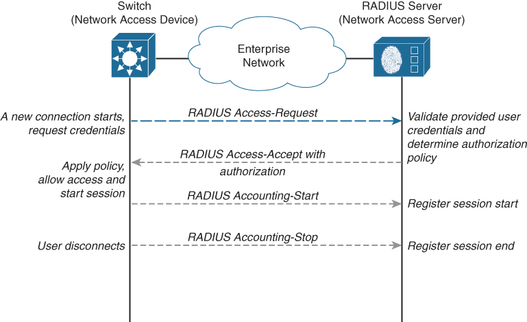
Figure A-5 Overview of RADIUS Protocol
The flow for RADIUS is relatively simple and consists of the following steps:
As soon as authentication is required, the Network Access Device (NAD, a client) sends an Access-Request RADIUS message to the Network Access Server (NAS). This message contains all required attributes for the authentication request, such as username, password, and other information.
The Network Access Server receives the Access-Request message and validates the NAD. Once the NAD is validated, it will look up the provided user and validate the password.
If the provided credentials are correct, the NAS determines the specific access policy and returns an Access-Accept message that includes the specific authorization policy by leveraging attribute-value keypairs. If the credentials are not correct, a simple Access-Reject message is sent back.
The NAD will parse and process the Access-Accept message and will apply the specific policy. The NAD will now send an Accounting-Start message to the NAS.
Once the session is closed, the NAD will send an Accounting-Stop message to the NAS to inform it of the closed session.
The RADIUS protocol was initially defined in RFC2058 in 1997. And although it is an old protocol, it is used in any campus network that uses IEEE 802.1X for Network Access Control. The reason for that lies primarily in the fact that the RADIUS packet is defined using an attribute-value-pair model. Besides a control-part inside the RADIUS packet, the actual data to be exchanged between NAD and NAS (and vice versa) is modeled around an attribute type, the length of the value, and the value itself. Each RADIUS message consists of a number of attributes and its corresponding values. For example, attribute type 6 represents the User-Name field.
And although the protocol only allows 256 unique attribute types, one of them is called the Vendor Specific Attribute type (VSA, value 26). This VSA is used to realize the extensibility and flexibility of the protocol. This VSA allows a vendor to define its specific list of attribute-value keypairs that can be used inside the RADIUS communication.
Cisco, with vendor ID 9, follows the recommended format protocol : attribute sep value for its vendor-specific attributes. Table A-1 provides a number of examples for a vendorspecific attribute.
Table A-1 Samples of Vendor-Specific Attributes
Example |
Description |
cisco-avpair= “device-traffic-class=voice” |
Assign the device into Voice class |
cisco-avpair= “ip:inacl#100=permit ip any 10.1.1.0 0.0.0.255” |
Apply an Access-list that only allows traffic to 10.1.1.0/24 |
cisco-avpair= “shell:priv-lvl=5” |
Assign privilege level 5 to this session |
This extensibility allowed for RADIUS to become the de facto standard for authentication and authorization services within network infrastructures, as each vendor is able to define extra attributes for its specific purpose. Over time, several extra attributes have been introduced by vendors. Within an Intent-enabled network, these VSAs allow the network operations team to define the policy at the RADIUS server (Cisco Identity Services Engine) and have the specific policy applied to the network port at the moment a device is connected and authorized.
Scalable Group Tags
Cisco introduced the concept of Source Group Tags (SGT; later known as Security Group Tags and now as Scalable Group Tags) with the introduction of Cisco TrustSec in 2007. In most network deployments, the enforcement of access policies is based on access lists that define which IP network is allowed to communicate with which destination and on which ports. Figure A-6 shows a typical enterprise network topology.
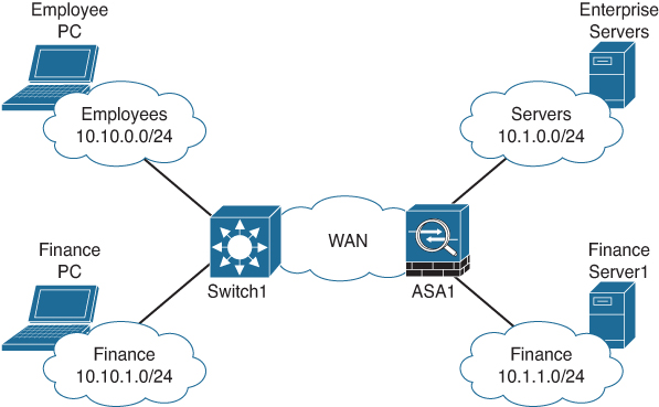
Figure A-6 Sample Overview of an Enterprise IP Network
In this example network, employees are connected to IP network 10.10.1.0/24 and are allowed access to the servers in 10.1.0.0/24. There is also a finance server network in IP network 10.1.1.0/24, and the finance employees are placed in IP network 10.10.2.0/24. If all employees are allowed access to the generic servers, but only the finance employees are allowed access to the finance server network, the access list on firewall ASA1 would be similar to that shown in Table A-2.
Table A-2 Sample Access List for ASA1
Source IP |
Destination IP |
Port |
permit/deny |
10.10.0.0/24 |
10.1.0.0/24 |
445,135,139 |
permit |
10.10.1.0/24 |
10.1.0.0/24 |
445,135,139 |
permit |
10.10.0.0/24 |
10.1.1.0/24 |
any |
deny |
10.10.1.0/24 |
10.1.1.0/24 |
445,135,139 |
permit |
With more applications being enabled on the network infrastructure, these access lists grow explosively in both length and complexity. Because of this complexity, the risk of unauthorized access (due to errors in the access list) is quite realistic. The principle of SGTs is to remove that complexity of source and destination IP addresses and define an IP-agnostic access policy. In other words, the access list policy is based on labels instead of IP addresses. Table A-3 shows the same access list policy, but then based on SGTs.
Table A-3 Sample SGT-Based Access List for ASA1
Source Tag |
Destination Tag |
Port |
permit/deny |
Employees |
Serv-Generic |
445,135,139 |
permit |
Emp-Finance |
Serv-Finance |
445,135,139 |
permit |
Any |
Serv-Finance |
any |
deny |
As you can see in Table A-3, the access list has become a policy matrix based on a set of tags or labels. Because the policy is now based on a tag, all employees can become part of the same IP network, which is also applicable to the servers. Figure A-7 shows the new network topology.
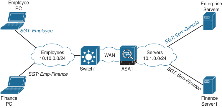
Figure A-7 Sample Topology of Enterprise with SGTs
The SGT concept is based on a central policy server (Cisco Identity Services Engine) in which the access policy is defined as a security matrix. The SGT assignment occurs when an endpoint is authenticated to the network; the SGT is added to the RADIUS authorization response. For servers, the SGTs are assigned manually within ISE, which could be based on a single IP address or a complete subnet.
Just as with VLANs, described in the section “VLAN” later in this appendix, the SGT is transported with the Ethernet frames received from the endpoint between Cisco switches.
Part of the Cisco SGT concept is that the same security matrix can be enforced on the access switch (to which the endpoints are connected). This means that the access switch has a downloaded Security Group Access List (SGACL) and enforces that on every packet that is received by the switch. This is, in fact, the enabler for microsegmentation (e.g., defining a micro security policy within a virtual network).
The Cisco TrustSec solution consists of more than SGTs, such as line-rate link encryption. Within an Intent-enabled Network, the concept of SGTs, in combination with a security matrix (defined in either Cisco DNA Center or Cisco ISE), is used to enable and implement microsegmentation.
Routing Protocols
Routing protocols are essentially the glue between different local networks. Routing protocols were developed and implemented so that different local networks could be interconnected to create a larger internetwork. Many books, such as Optimal Routing Design by Russ White, have already been written on routing protocols that provide in-depth coverage of the protocols, their mechanisms, and their technologies.
This section is not intended to provide a complete overview of the individual routing protocols currently available, but rather provide an overview of the concept of how routing protocols are used to glue local networks into a larger network and how that is related to IBN.
Concept of Routing Protocols
Common routing protocols, such as IS-IS, BGP, OSPF, and (E)IGRP, all have a single goal in common: they aim to provide a method to determine how a packet with a specific destination IP needs to be forwarded to which link. All these protocols aim to provide the most optimal route through this interchain of connected networks. Figure A-8 shows a sample network topology where several networks are interconnected with each other.
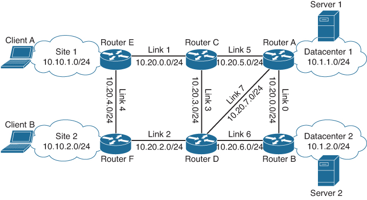
Figure A-8 Sample Network Topology
In this network, a sample enterprise, two campus sites (Site 1 and Site 2) are connected via a myriad of connected links to the two datacenters (Datacenter 1 and Datacenter 2). To allow communication from Client A to Server 2, all routers in the network would need to know how to forward packets back and forth. In other words, they need to be aware of how a specific network is reachable (reachability) and which link to use to forward a packet (the topology of the network). And as there are loops in the network for high availability, the routers also need to keep that topology loop-free.
One option would be to configure all site networks statically on all routers so that the routers know the topology and the networks. But static routes do not scale well and can provide problems in case of link failures.
Routing protocols are designed to solve just that; they learn the topology and reachability information about the connected networks dynamically. There are two mechanisms for how routing protocols can learn the topology and reachability—link-state and distance-vector.
Distance-Vector
In a distance-vector routing protocol, each router in the network periodically shares all the networks it knows about with the associated distance (cost) to reach that network. The cost of a direct-connected network is, of course, the lowest. A distance or cost could be the hop count (for example, how many hops need to be taken before it can reach that network).
If a router receives a network update from a neighbor with a better cost, it will update its internal network database (topology) and will forward its updated network knowledge in the next update.
Over time, each router has learned all networks it can reach with the associated cost. As soon as a packet is received, its destination IP address is looked up in the topology database and is forwarded to the neighboring router with the least cost.
The distance-vector mechanism can be compared to road signs with the different cities (destinations) along the highway. If you were to drive to a specific city that required multiple highways, you would follow the road signs at each highway junction (router) to reach your destination.
The disadvantage of a distance-vector routing protocol is that it does not (always) take into account what the bandwidth and utilization of that link is. In the highway example, the distance-vector does not include a means to inform whether the highway is a two-lane road or a six-lane highway. It could result in packets arriving slowly because of congestion (traffic jams).
Link-State
The other mechanism that can be used to learn the topology and reachability is link-state. In contrast to distance-vector, the routers initially determine on which links they have neighboring routers (checking for reachability over a link). This reachability is checked periodically. Once reachability is established, the router floods its information about neighbors and networks (link-state) to all its connected neighbors. This leads to allrouters having received information from all other routers and connected networks. Once this information is received from all routers in the network, each router will use an algorithm (Dijkstra’s shortest path) to determine what the most optimum route is for each network. If a link fails, the link advertisements are sent again, and the topology is recalculated.
Effectively, link-state routing protocols maintain a database with all routers, the (connected) links to other routers, and the connected networks for each router, and use that to determine the topology and reachability.
Link-state routing protocols are common in smaller networks where the knowledge of all routers and connected networks does not lead to scalability and resource problems; if the number of routers in the network becomes too high, the cost of calculating the optimal route and maintaining that database takes too many resources.
A common example of the link-state mechanism is how a GPS navigation system determines the route from A to B within a city. Its map information allows creating a topology of all the roads (links) and their interconnections (routers) within the city. And the shortest path algorithm allows for determining the shortest path between two random points within the city limits. However, maintaining a full topology of all streets and their interconnections within a continent would be too large, and calculating the shortest route would take too long. Therefore, in these situations, most GPS navigation systems use hierarchies (network topologies on top of network topologies) to optimize the resources.
Every routing protocol used within a campus network is based on either one of these two mechanisms. For example, Open Shortest Path First (OSPF) and Integrated System-to-Integrated System (IS-IS) are based on the link-state mechanism, whereas Border Gateway Protocol (BGP) is based on the distance-vector mechanism. Cisco introduced Extended Interior Gateway Routing Protocol (EIGRP) as a combination of link-state and distance-vector mechanisms, which provides some unique improvements.
And although it does not matter which protocol is used for a traditional campus network, the choice of routing protocol does matter for an Intent-Based campus network.
In both a non-fabric as well as an SDA-based campus network, multiple virtual networks are deployed within the network. This means that the reachability and topology information needs to be exchanged within those virtual networks. The most commonly deployed routing protocol for that is BGP.
An SDA-based network adds the requirement for a routing protocol in the underlying switching infrastructure, as each link between the switches is IP-based. The most common routing protocol for the underlay network is IS-IS, where the IS-IS network itself is terminated at the border nodes of the fabric.
Software-Defined Access
Software-Defined Access is the next evolution of campus networks and combines several common technologies (IEEE 802.1x, VRF-Lite, RADIUS, and SGT) with relatively new technologies for the campus network environment. Chapter 5, “Intent-Based Networking,” described the design and concept of an SDA-based campus network. The following sections describe the two new technologies used within SDA.
VXLAN
Virtual eXtensible Local Area Network (VXLAN) is a technology that originates from the datacenter networks. The classic VLAN technology is restricted to 4096 different VLANs, thus limiting the datacenter network to 4096 logical Layer 2 networks. Another limitation of a Layer 2 network is that stretching it over multiple datacenters will introduce several complications, such as latencies, split-brain, and non optimal traffic flows. To overcome these problems, VXLAN was developed and introduced in the datacenter.
VXLAN itself is a network virtualization (overlay) technology that allows you to embed any Layer 2 packet into a logical network (virtual network id). VXLAN uses UDP to encapsulate those Layer 2 packets and forward them to the proper destination. The receiving switch decapsulates the original Layer 2 packet from the VXLAN packet (UDP) and forwards it locally as if it were a single logical network (like a VLAN). Figure A-9 provides an overview of how VXLAN is used to transport information across a different IP network.
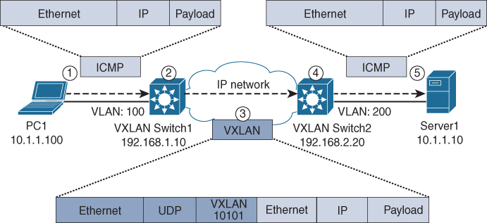
Figure A-9 Output from the SIMPLE Program
In Figure A-9, PC1 and Server1 are on the same logical IP subnet (10.1.1.0/24) but are physically separated by a different IP network. The VXLAN switches allow the devices to connect and communicate with each other. For example, PC1 sends a ping (ICMP) packet to Server1. The following flow happens:
PC1 sends an ICMP packet with destination IP address 10.1.1.10 onto the Ethernet connection to VXLAN Switch1.
VXLAN Switch1 receives the incoming ICMP packet from PC1 on VLAN 100. VLAN100 is configured to forward packets onto VXLAN 10101. This means that VXLAN Switch 1 will embed the complete ICMP packet into a new VXLAN network with VXLAN identifier 10101 (purple). VXLAN Switch1 uses a controlplane lookup to determine the destination of the VXLAN packet. For that lookup, it uses (in case of a Layer 2 VXLAN) the destination MAC address of the original (yellow) packet. Based on the control-protocol lookup, the destination IP will be 192.168.2.20, and VXLAN switch 1 will forward the packet based on the routing tables of the IP network.
IP Network will forward the new (purple) VXLAN packet through its network to its destination, 192.168.2.20.
Upon receiving the VXLAN packet, VXLAN Switch2 will decapsulate the VXLAN packet. Based on the VXLAN Identifier (10101) and its configuration, it knows it needs to forward the packet to VLAN200. Again, a control-protocol lookup (of the original yellow destination MAC address) will be used to determine to which interface the packet needs to be forwarded. Once the lookup is successful, VXLAN Switch2 will forward the original (yellow) packet onto the wire to Server1.
Server1 receives the original ICMP packet as a normal packet, and the response sent to VXLAN Switch2 will have to take the same path.
For PC1 and Server1, the complete VXLAN communication is transparent. They have no insight or knowledge that a separate IP network is in between them. An SDA network within the campus behaves in the same manner, where the switches where endpoints reside are named edge nodes, and the node where traffic is leaving the fabric is called a border node.
VXLAN itself allows for 16 million (24 bits) different logical virtual networks, identified as virtual network IDs. Within SDA, the VXLAN identifier is the same as the virtual network ID defined within Cisco DNA Center, which theoretically allows for up to 16 million virtual networks in a single campus fabric.
VXLAN itself is designed as a data-path protocol; in other words, its scalability and performance lie in the quick encapsulation and decapsulation of data-packets. A separate control-protocol is required to determine where each VXLAN packet needs to be forwarded.
LISP
SDA leverages VXLAN technology to define overlay virtual networks and transport them via an underlay network within a campus fabric. But VXLAN is a datapath technology; it relies on a control protocol for lookups and determining which destination IP address is used within the underlay network. Within SDA, Locator/Identifier Separation Protocol (LISP) is used as the control protocol.
LISP was originally an architecture (and protocol) designed in 2006 to allow a more scalable routing and addressing scheme for the Internet. Already at that moment, the number of IPv4 networks in the database of routers on the Internet was exponentially growing. The primary causes for that were the fact that there was an exponential increase in smaller IP subnets announced on the Internet, as well as that more organizations would be connected (and thus announced) via multiple providers.
Effectively in today’s Internet, for each public IP network, the network and how to reach that network (location) is known. This is an integral part of the distance-vector routing protocol used on the Internet. And because every router on the Internet needs to know how to reach each network, each router effectively has a large database of networks and locations (how to reach those networks). And as the number of networks grows, the required resources to manage that increase too, which can also result in slower routing table loading times after a reboot or disconnect of a link.
LISP was designed to reduce that increase in complexity and increase in resource requirements. Conceptually, LISP achieves that reduction by both separating the IP networks (named endpoint identifiers [EID] in LISP) and how to reach those networks (via Routing Locator [RLOC] in LISP) information and moving that information into a smaller number of large database or mapping servers.
Routers in the network would inform that mapping server which endpoint identifiers (EID) were reachable via that router. And at the same time, if they need to know where to forward a specific packet to, they would perform a lookup in that LISP server to find which RLOC would be responsible for that network and then forward the packet to that specific RLOC. This results in a smaller, on-dynamic table on each router inside the network, while retaining full knowledge of where each EID (IP network) is located. Figure A-10 shows a (simplified) diagram of a larger Internet-network where two ISPs are used to connect several IP networks.
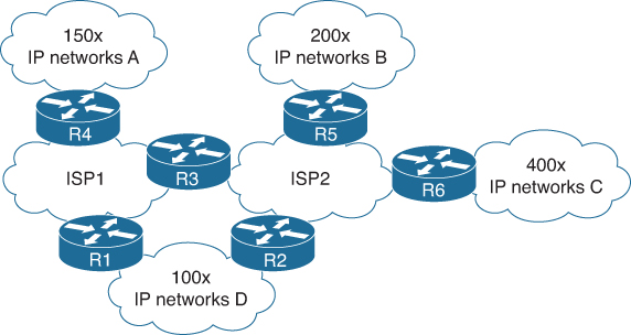
Figure A-10 Traditional Sample Interconnected Network
In the traditional (and today’s Internet) network, each router would maintain a routing table containing all the networks and how they are reachable, such as Table A-4 for R6.
Table A-4 Routing Table for Router R6
IP Network (EID) |
Reachable via (RLOC) |
400x IP Networks C |
Directly connected |
150x IP Networks A |
ISP2-R3 |
200x IP Networks B |
ISP2-R5 |
100x IP Networks D |
ISP2-R2 |
100x IP Networks D |
ISP2-R3 ISP1-R1 |
Router 6 alone already has 950 routes in its database, with this relatively simple design. Every other router in the same IP network would have 950 routes, resulting in 5700 IP networks. Imagine what would happen with the numbers if this network would scale up to the size of the Internet with tens of thousands of service providers and enterprises.
Each router on the Internet would require the resources to maintain that kind of table.
With a LISP-based network, the network from Figure A-10 would look like Figure A-11.
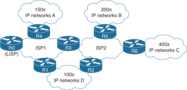
Figure A-11 Sample Interconnected Network with LISP Enabled
With LISP configured on the network, each router would provide its location identification (RLOC) and the connected networks (EID) to the LISP mapping server on R0. Table A-5 shows the mapping table on Router R0.
Table A-5 LISP Mapping Table for Router R0
IP Network (EID) |
Reachable via (RLOC) |
400x IP Networks C |
ISP2-R6 |
150x IP Networks A |
ISP2-R3 |
200x IP Networks B |
ISP2-R5 |
100x IP Networks D |
ISP1-R1 or ISP2-R2 |
The table itself looks similar to the table of Router R6. But instead of having each router maintaining that full table of IP networks, only R0 will maintain that table. Each router will only maintain a cache of table entries to reduce the number of routing tables. If from IP Network C most traffic flows to IP Networks A and B, the routing table on router R6 would only have 350 routers instead of 950 (full routing table). This results in a reduction of required resources on router R6.
LISP itself also contains other technologies and concepts to reduce the number of IP networks (prefixes) on such a network, such as tunneling traffic. But within SDA, the concept and principle of the LISP mapping server is primarily used within the campus fabric.
Within SDA, the LISP mapping server is named the control node. EIDs are the endpoint IP addresses (or MAC addresses for a Layer2 Virtual Network), and the RLOC information contains the lookback address of the edge node to which the device is connected. This mapping information is used to encapsulate the endpoint’s traffic in VXLAN packets sent over the underlay of the fabric.
Classic Technologies
A non-fabric deployment leverages several classic technologies to enable an Intent-Based Network. The sections that follow describe the concepts of these classic technologies.
VLAN
One of the best known and most used technologies in a campus network is the virtual local area network (VLAN). VLANs are used to isolate several physical Ethernet connections into logical Layer 2 domains. The isolation could be because of a business requirement (isolation of printers from employee workstations or guest users), or to create smaller broadcast domains for manageability. The VLAN technology is defined in IEEE 802.1Q standard and is a Layer 2 network technology.
Traditionally, as shown in Figure A-12, every Ethernet device in the same physical network can communicate with each other. In other words, PC1 can freely communicate with PC2, the server, and other devices on the same switch.

Figure A-12 Single Ethernet Domain with No VLANs
If, for any reason, PC1 and Server1 are part of the financial administration department, and PC2 and PC3 would not be allowed access, without VLANs these two devices would need to be connected to a different physical switch. Although this is a valid option, it is not scalable and is expensive. A VLAN is used to create logical switches within that single physical switch. To achieve that, each Virtual LAN is provided with a unique identifier, a VLAN ID. This VLAN ID ranges from 2 to 4095. VLAN ID 1 is the so-called default VLAN and is used for switches that do not support VLANs. Figure A-13 shows the same physical topology but now with a VLAN for Finance (red) and a VLAN for Employees (blue).
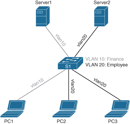
Figure A-13 Switch Topology with Two VLANs
At this moment, the devices that are configured with VLAN 10 (Finance) can only communicate with each other, and those that are connected to VLAN 20 (Finance) can only communicate with each other. Because of this isolation, VLAN 10 and VLAN 20 will never communicate with each other. That also means that PC1 cannot communicate with Server2, because it is on a separate VLAN and thus a separate logical Layer 2 network. Only if the switch (or firewall or router) would have IP addresses in both VLANs, routing is possible on Layer 3 and communication can occur.
The IEEE 802.1Q standard also describes how the Layer2 isolation principle works when multiple switches are connected and the Layer 2 isolation should be spanned across the switches. Figure A-14 shows the same topology, but now PC3 is connected to a separate switch.
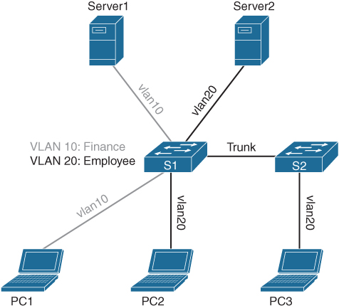
Figure A-14 Topology with Two Switches and Two VLANs
For PC3 to be able to communicate with Server2, the two switches are connected with a special IEEE 802.1Q interface. Within Cisco switches, it is called an Ethernet trunk. The Ethernet frames sent and received between the two switches also include the VLAN Identifier as a tag. It is also known as “tagged traffic.” That way, if an Ethernet frame is received by S1 with Tag20, S1 knows which VLAN that Ethernet frame belongs to, so S1 can forward it to the appropriate logical network. The format of such an Ethernet frame is described in the IEEE 802.1Q standard.
In summary, VLANs are commonly and widely used technology for isolating Layer 2 networks. VLAN interfaces on switches (or firewalls or routers) are used to connect the different isolated Layer 2 networks for interconnectivity. Within an Intent-Based Network, VLANs are used in a nonFabric deployment to isolate the different virtual networks.
STP
Spanning Tree Protocol (STP) is a technology that is used to prevent loops in Ethernet networks. Although it was originally designed as a hack1 to be able to create a single path from two nodes across multiple ethernets, STP has become one of the most common and widely deployed protocols in the campus network. The concept of STP is based on the premise that there can only be a single path between nodes in a redundant connected Ethernet network. To accomplish that premise, STP operates at Layer 2 (Ethernet) and builds a logical topology (based on a tree) on top of physically connected redundant switches. Figure A-15 displays a small switches topology.
1 According to an interview with Radia Perlman, the designer of Spanning Tree, found at https://xconomy.com/national/2019/07/08/future-of-the-internet-what-scares-networking-pioneer-radia-perlman/

Figure A-15 Small Switch Topology
If STP would not be enabled in the above network topology, a broadcast storm would follow very soon. Suppose PC1 sends an Ethernet broadcast out to discover the IP address of Server1. That broadcast would be received by switch S2. S2 would, in turn, send that broadcast to S1 and S3. Both switches would, in turn, send that same broadcast to their uplinks. That would result in the broadcast S2 sent originally being received back twice (one via the path S3 -> S1 -> S2 and the other via the path S1 -> S3 -> S2). Because ethernet is a layer2 protocol, it has no concept of a time to live (or hop count), and within a matter of seconds the links between the switches become congested with a single broadcast.
Because STP is designed to only allow a single path for Ethernet packets, broadcast storms are prevented if STP is configured. STP achieves this design principle by periodically sending out special bridge packets to each interface, with an identifier of that switch and other information. As soon as such a packet is received by any other switch, that switch will stop processing all data and start a Spanning Tree calculation process. That process involves all switches in the network (which will, of course, also stop traffic). The received bridge packets are used to logically determine which switch will be the root of the Spanning Tree (the switch with the lowest MAC address and lowest priority). After the root has been determined, each switch builds up a topology of the network and uses the shortest path to determine what the most optimal path is to that root-switch. Once the shortest path has been calculated and determined, all other interfaces via which the root switch has been learned will be blocking inbound traffic to prevent loops in the network. The method used in STP is similar to the process of the link-state mechanism described in the routing protocols section.
Figure A-16 displays the same network topology but with Spanning Tree configured and active with S1 as the root.
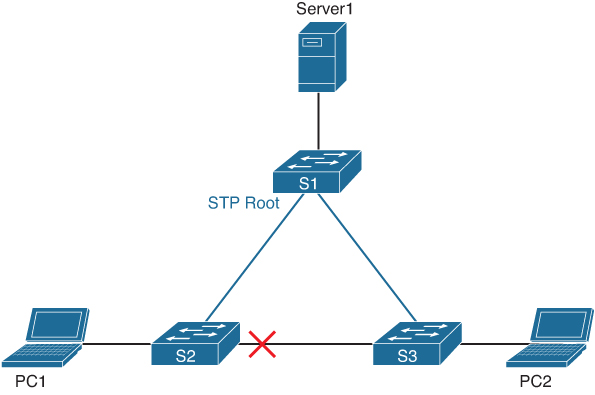
Figure A-16 Small Network Topology with Spanning Tree Enabled
In this figure, the links in blue are active links, whereas the red X marks that interface in blocking.
With the same example in Figure A-16, if an Ethernet broadcast would be received from PC1 by S2, S2 would only forward the broadcast to S1. S1 would, in turn, send the broadcast out to S3. S3 would send that broadcast to S2, but because S2 has blocked that interface, it will not forward that packet out. The broadcast storm has been prevented.
Because STP is a Layer 2 protocol (and is enabled by default), STP can lead to odd behaviors when a switch is introduced to the network. It could even lead to the new switch being the root of the network, with odd performance problems and behaviors as a result.
Within the original (and formal IEEE 802.1D standard) STP, the switch would block all traffic for 30 seconds. Because this block would also occur when a PC connects to the network (the switch does not yet know that it is a PC or a switch), it led to connectivity issues and timeouts for obtaining an IP address.
To solve that problem, IEEE introduced Rapid Spanning Tree Protocol (RSTP) as IEEE 802.1w. In this standard the timers were reduced from 30 seconds to three times a hello message, reducing the blocked time to approximately 6 seconds. This resulted in more reliable service to the enterprise with fewer network connectivity problems.
Besides RSTP, Cisco implemented a proprietary optimization, where RSTP could be deployed per VLAN. This protocol was called RPVST. Because RSTP would be run per VLAN on a campus network, the load of the traffic across two distribution or core switches could be shared by having one core be the STP root for a number of VLANs and the other core be the root for the other VLANs. An added benefit of RPVST is that if a link comes up in, for example VLAN 100, only that VLAN would start its STP process and block traffic. However, because RPVST requires more memory and CPU in a switch (a topology per VLAN needs to be maintained), almost all Cisco Catalyst switches have restricted the number of instances to 128. This means that if a campus network has more than 128 VLANs, STP will not function for some VLANs. It is random which VLANs will not work.
Another improvement in STP is called Multiple Spanning Trees Protocol (MST), based on IEEE 802.1s standard. It effectively is a mix between STP and PVSTP, where an instance of STP is configured for a group of VLANs, thus restricting the number of instances. Most Cisco switches support a maximum of 63 MST instances.
In general, STP seems like a very good and solid technology to solve loop problems in the network. However, more modern technologies, such as virtual PortChannel (vPC) and Multichassis EtherChannel (MEC), remove the loops from a network completely, which removes the need for STP. Recommended practice dictates that non-SDA Intent-Based Networks remove STP as a protocol completely to reduce the complexity of the network, as long as there are no loops in that campus network. If there are loops in the network, then use MST as Spanning Tree Protocol.
VTP
VLAN Trunk Protocol (VTP) is probably one of the most underestimated protocols in the campus networks. VTP is a Layer 2 network protocol that can be used to propagate the VLAN creation, modification, and deletion of VLANs across switches. VTP is a Cisco proprietary protocol. The most recent version of the VTP protocol is version 3, and it has a lot of improvements.
The concept of VTP is relatively simple. VTP is based on a client-server approach within a single management domain. Within a single management domain (defined by a domain name), all VLANs are managed on a VTP server. After each change, the VTP server will inform the VTP clients of that change by sending an Ethernet update. All VTP clients within that same domain will receive and process that update. Figure A-17 provides a network that has VTP enabled.

Figure A-17 Overview of VTP Domain
The example in Figure A-17 displays that there is a network with a VTP Server for a domain named “campus.” As soon as a network operator creates a new VLAN on that switch with the VTP Server role, the switch will generate a VTP update message and broadcast the message to every connected interface (indicated by the number ➀).
As soon as a VTP client receives a VTP update message, it performs two validations. The first validation is if the update is meant for its management domain. The second validation is to check the revision number inside the message to see if the update is newer than the latest version known to the VTP client. If both validations are correct, the update message is processed and the change is replicated on the switch. The VTP client will then forward the message to every connected interface (indicated by the number ➁).
If both validations fail, the VTP client ignores the messages for its own configuration but will broadcast it to all connected interfaces (indicated by the number ➂).
VTP is a powerful protocol that makes the management of VLANs on a large network easy. But the power comes with a cost. VTP is a Layer 2 protocol, and as with any Layer 2 protocol, it is enabled by default. So in case a switch in the network is replaced with a new switch (or one from a lab environment) and that switch has VTP configured as a server, in the same domain, and has a higher revision number than the current VTP server, all VTP clients will use that VLAN database as leading. If that new switch then also has no VLAN configured (write erase does not delete the VTP configuration), all VLANs will be removed from the network.
Because this has happened in the field many times, most enterprises disable VTP to prevent these outages. Although it is a valid reason, the true root cause of such incidents is, of course, that the switch that is placed in the network has not been configured correctly.
With VTP version 3 (the latest version), it is possible to define a primary and secondary switch as VTP server, which prevents these types of problems as well.
For a non-Fabric Intent-Based Network, VTP can be used to deploy VLAN changes via a single change on the distribution switch, which will make the deployment of new intents much easier.
Analytics
Besides technologies used for the configuration of the campus network, several technologies are used to monitor the correct operation of the network. Within an Intent-Based Network, the analytics component is an integral part of how the campus network is operated and managed. The sections that follow describe the technologies (both existing and new) used for the analytics component of an Intent-enabled network.
SNMP
One of the most common protocols used within network management is Simple Network Management Protocol (SNMP). Do not be fooled by the name of the protocol in terms of management. The protocol itself might be simple, but the implementation, configuration, and operation using SNMP can become complex and can have (if misconfigured) a huge impact on the performance of the network.
SNMP is based on the concept that there is a management network, a network management station, and a set of managed devices. Managed devices have SNMP agents installed, and an SNMP manager is running on the network management station. Figure A-18 provides an overview of the concept.

Figure A-18 Conceptual Overview of SNMP
SNMP consists of two different methods of communication:
SNMP requests: Used by the network management station to either request information from a managed device (GetRequest) or to set a value on the device (a SetRequest). As an example, the network management station sends a request for the CPU load to the managed device (using UDP). The managed device receives the request, validates the authenticity of the request, and then sends the response back. This is represented in the figure as the blue lines.
SNMP traps: Used by the managed device to inform the network management station that something has happened. For example, the managed device detects that the CPU of the device is too high; it can send an SNMP trap to the network management station to inform that the CPU is high.
Because SNMP is based on UDP (no confirmation), it relies on the resilience of the network for the trap to be received by the network management station.
As stated, the concept of having a request-response method, where specific information elements can be requested and the concept of receiving a trap when something is wrong, is indeed simple. However, the method of how to specify and configure what information is to be requested is when SNMP becomes complex.
SNMP uses Object Identifiers (OID) to uniquely identify every item that can be requested via SNMP. That means that there is a unique identifier for the operational status of every individual interface of a switch, and for every route entry in a router, there is a unique identifier.
To be flexible and extensible as a network management protocol, the OIDs within SNMP are grouped in a tree, where each node and element in the tree is identified by a decimal value. The OID 1.3.6.1.2.1.2.2.1.8 translates to the operational status of interface 1. Management Information Blocks describe (in a specific language) how the OIDs are organized. The same example above would translate to 1(iso).3(org).6(dod).1(internet).2(mgmt).1(mib-2).2(interface).2(ifTable).1(ifEntry).8(operStatus).
The concept of a tree enables different vendors to define their specific subtree in the same hierarchy. The MIB files are used by the network management station to translate text-based information to the OID to be requested. And this is one of the aspects that makes the configuration of SNMP complex, because every information element that the management station wants to monitor needs to be configured. There are, of course, templates, but the configuration of SNMP requires some manual configuration.
Also, the impact of SNMP on the managed devices can be quite high, because the managed device is for SNMP requests effectively a server. That means that the CPU of the managed device (usually the CPU is very slow compared to switching in optimized ASICs) has to handle these requests, and thus if many requests are sent to the switch, the CPU can easily go to the max.
Although later versions of SNMP support requests in bulk (instead of a single SNMP request per information element), many SNMP management tools still use the single request method. This means that the minimal information for every interface on a stack of four 48-port Cisco Catalyst 3650 switches results in 1152 (6 * 4 * 48) requests. When the management station sends those out in a single burst, it is a serious impact to both the CPU of the switch and the number of connections generated.
The security of SNMP differs from the three versions that are currently available. SNMPv1 is the first version and had no security; everybody could send and receive requests. SNMPv2 introduced the concept of communities, where each community was used both as a pre-shared key for authentication and authorization (the SNMP community would be either read-only [only GetRequests] or read-write [GetRequests and SetRequests]). SNMPv3 is the latest version and includes modern encryption and hashing methods for authentication and authorization. The advantage of SNMPv3 is that it is much more secure but does have a higher impact on the CPU.
In summary, the name Simple Network Management Protocol is a bit misleading. The protocol itself is simple, but the configuration and management are much more complex. Also, the impact of SNMP on the individual devices within a network is quite high, specifically if multiple management stations start to request the same information.
With an Intent-Based Network, the network infrastructure is business critical, which requires monitoring of much more than just the interface status, which results in an even higher impact on the network and network devices. Therefore, it is not recommended to use SNMP for an Intent-Based Network. As explained in Chapter 4, “Cisco Digital Network Architecture,” Model-Driven Telemetry is a technology that suits Intent-Based Networking better. Its concept is explained later in the section “Model-Driven Telemetry.”
Syslog
Syslog is a technology that originates from the UNIX and mainframe systems environment. Its system is based on having a central (and unified) environment where each process and application could log messages to. The Syslog environment would then distribute the messages to different files, a database, or via the network to a central Syslog server, so that the logging of all workstations is centralized.
Syslog within a network infrastructure operates in the same manner, and commonly uses RFC5454 (The Syslog Protocol) for that. It uses the same Syslog standard, and network devices send their log messages to a central Syslog server. RFC5454 follows the principle that each Syslog message is sent as a single packet to a central Syslog message. Each Syslog message has several fields and descriptors that can be used to provide structured information. The fields follow the Syslog message format that originated from the UNIX environment. Table A-6 provides an overview of all the Syslog fields.
Table A-6 Overview of Fields in a Syslog Message
Syslog Field |
Description |
Facility |
The facility originates from the UNIX environment and explains what the originator was (kernel, user, email, clock, ftp, local-usage). Most network devices log using facility level local4. |
Severity |
A numerical code that describes the severity, ranging from 0 (emergency) to 7 (debugging). |
Hostname |
The host that sent the Syslog message. |
Timestamp |
The timestamp of the Syslog message being generated. |
Message |
The Syslog message itself. For Cisco devices, the Syslog message follows the format %FACILITY-SEVERITY-Mnemonic: Message-text. Both the FACILITY and the SEVERITY are often the same as the Facility and Severity of the Syslog protocol message. The Message-Text is the actual text of the Syslog message. |
Mnemonic |
The mnemonic is the OS-specific identifier of the Syslog message; for example, CONFIG_I within IOS devices informs about a configuration message, and the code 305012 specifies a teardown of a UDP connection on a Cisco ASA firewall. |
Within networking, Syslog messages can be compared to the SNMP traps, as they “tell” the Syslog server and network operator what is happening on the network. There are two advantages that Syslog provides over SNMP traps. The first is that there are many more Syslog messages compared to SNMP traps. In comparison, a Catalyst 6500 running IOS 12.2 has approximately 90 SNMP traps but over 6000 different Syslog event messages.
The second advantage is that Syslog provides much more granularity, as the log level, log severity, and message details can be used to create filters and determine which messages need response to.
Several solutions exist that rely on Syslog for monitoring network infrastructures. The most commonly known concept is a Security Incident Event Management (SIEM) system. It collects Syslog information from many sources and uses smart filters and combinations (which you have to define) to detect anomalies in the network.
In general, Syslog is used for two flows within the operation of the network. The first is by looking at the content of the Syslog messages themselves. By looking at the messages, information is provided on what’s happening on the network. The Syslog message in Example A-4 is providing information that a MAC address has been moved between two interfaces (which in this case is logical because it is a wireless client that roamed to another AP) and that the user admin changed the running configuration.
Example A-4 Sample Syslog Messages
Jul 18 2019 14:27:01.673 CEST: %SW_MATM-4-MACFLAP_NOTIF: Host 8cfe.5739.6412 in vlan
  300 is flapping between port Gi0/6 and port Gi0/8
Jul 18 2019 14:29:08.152 CEST: %SYS-5-CONFIG_I: Configured from console by admin on
  vty0 (10.255.5.239)
<166>:Jul 18 14:41:03 CEST: %ASA-session-6-305012: Teardown dynamic UDP translation
  from inside:10.255.5.90/60182 to outside:192.168.178.5/60182 duration 0:02:32
<166>:Jul 18 14:41:03 CEST: %ASA-session-6-305012: Teardown dynamic UDP translation
  from inside:10.255.5.90/61495 to outside:192.168.178.5/61495 duration 0:02:32
Another common use case for network operations is to look for variations in the number of log messages produced by the network infrastructure. For example, suppose that the network generates an average of 500 log messages per minute, and at one moment in time the average spiked to 3000 log messages per minute. That spike is effectively the network telling the operator (via log messages) that something is happening on the network.
In summary, SNMP is a widely and commonly deployed technology for monitoring behavior on IT devices, whereas Syslog is specifically used for monitoring what is happening within the network infrastructure. The technology is used by the analytics component within the Intent-Based Network irrelevant of the technology to deploy the intents.
Model-Driven Telemetry
In today’s network infrastructures, SNMP is commonly used to get telemetry data (values to determine the operational state and statistics of the network, such as interface statistics). Besides that this method of obtaining telemetry data results in spikes on the CPU, SNMP is limited to only provide telemetry data on the network infrastructure layer. It is not capable of providing telemetry data on how long it takes a user to connect to the network.
To overcome these two problems, Model-Driven Telemetry is used to transport telemetry data from network devices to a network management system. Model-Driven Telemetry uses a subscription-based approach, where the roles of client and server are reversed. The network management system (for example, Cisco DNA Center, as a client) is not hammering the network switch with single telemetry data requests to the network switch (the server); within Model-Driven Telemetry, the network management system requests a subscription to telemetry data from the switch. In return, the switch (as a client) will connect to the network management system (server) and provide data to that subscription. Figure A-19 provides a conceptual flow of this concept.
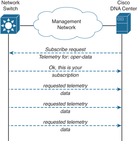
Figure A-19 Conceptual Flow of Model-Driven Telemetry
Within Model-Driven Telemetry, Cisco DNA Center (for example) requests a subscription for telemetry data of the network switch. It is not possible to subscribe to all data in a single subscription. In this example, Cisco DNA Center requests for oper-data (like CPU load, memory utilization) and asks for periodic subscription. The network switch validates the request and generates a subscription ID, which will be returned as a response to Cisco DNA Center.
After that initial request, the network switch will periodically push the telemetry data (of that subscription) to the subscriber—in this case, Cisco DNA Center.
This subscription model provides several benefits in comparison to SNMP. The request for telemetry data is only sent once. After that, the switch will send the requested telemetry data periodically (or on a change, which is another subscription option within MDT). Effectively, the switch has become the client, and the switch is not overloaded with many SNMP requests. The data is sent in a bulk stream update to the management station.
MDT uses the subscription model to optimize the flow and reduce the impact and load on the network devices. But another difference is that the data that can be subscribed to is based on open model specifications. Instead of having individual object identifiers for each data element, a model of the telemetry data is defined and used as part of the request. These models are based on YANG data models. YANG is an open data modeling standard that is used by the network industry to allow for a vendor-independent method (and model) for configuring network devices. The YANG models are publicly available on GitHub and are made available per IOS-XE release (as there can be differences between versions).
Model-Driven Telemetry has become available for all switches since Cisco IOS-XE 16.6.1. Newer releases also include support for Cisco routers. Over time, all Cisco devices running IOS-XE will support Model-Driven Telemetry. It is the primary technology used within Cisco Digital Network Architecture to provide data to the analytics component.
NetFlow
NetFlow is a technology developed by Cisco that is used to collect metadata about the traffic flowing through the network. NetFlow’s concept is that on strategic entry and exit points in the network (for example, the first Layer 3 hop in the campus network), an exporter is configured. The exporter collects statistics for every connection that flows through that device. The statistics usually consist of source and destination IP information, the time of the connection, and the number of bytes sent and received. Periodically the exporter sends these statistics as flow-records to a collector.
Figure A-20 shows the principle of NetFlow.
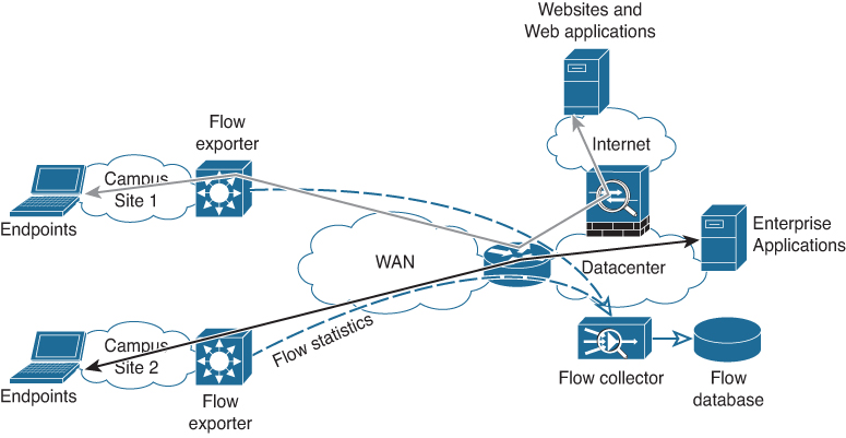
Figure A-20 Sample Topology with NetFlow
In Figure A-20, endpoints from different campus locations access applications on the Internet (red flow) and the enterprise applications (green flow). The distribution switch in both campus locations exports flow statistics to the flow collector. Operators connect to the flow collector to see what flows run through the network.
Because NetFlow collects statistics at a higher frequency than SNMP is commonly polled and it collects metadata on the applications and protocols used, NetFlow provides an excellent technology to determine which applications run over the network and how much bandwidth is used for specific applications and links.
Most collectors save the flow information in a database so that the flow information is retained for troubleshooting and forensic analysis (what happened during a specific network outage). Both use cases are an integral part of the analytics component of Cisco Digital Network Architecture, and NetFlow is used as one of the technologies to provide extra information.
Summary
A campus network designed, deployed, and operated based on Intent-Based Networking uses several technologies. The concepts of most technologies have been described in the previous paragraphs. Table A-7 provides an overview of these technologies and which technology is used within each type of deployment for Intent-Based Networking in the campus network.
Table A-7 A Summary Overview of the Technologies and Their Roles in Intent-Based Campus Networks
Technology |
SDA Fabric |
Classic VLAN |
Role |
Network PnP |
✓ |
✓ |
PnP is used for LAN Automation and day0 operations. |
VRF-Lite |
✓ |
✓ |
VRF-Lite is used for the logical separation of virtual networks. |
IEEE 802.1X |
✓ |
✓ |
Used to identify and authenticate endpoints connecting to the Intentenabled network. |
RADIUS |
✓ |
✓ |
RADIUS is used for the authentication and authorization of endpoints between the central policy server and the network access devices. |
SGT |
✓ |
✓ |
Security Group Tags are used for microsegmentation. |
Routing protocols |
✓ |
✓ |
Used to exchange reachability and topology information per virtual network; in case of SDA also used for the underlay network. |
VXLAN |
✓ |
|
Used to isolate and transport virtual networks over the underlay network. |
LISP |
✓ |
|
Used as control protocol within the fabric. |
VLAN |
|
✓ |
Used to logically isolate networks on Layer 2, similar to VXLAN on SDA. |
STP |
|
✓ |
Preferably not used at all, but if required, used to prevent Layer 2 loops in the network. |
VTP |
|
✓ |
Used to easily distribute VLAN information across the campus network. |
SNMP |
✓ |
✓ |
Used for basic monitoring of devices not supporting Model-Driven Telemetry. |
Syslog |
✓ |
✓ |
Used for monitoring and analytics within the network. |
NetFlow |
✓ |
✓ |
Used to analyze the flows and application detection in the campus network. |
Model-Driven Telemetry |
✓ |
✓ |
Used by network devices to provide intelligent telemetry data to the analytics component of the Intent-Based Campus Network. |