
9
![]()
Assessing Teachers from student scores
On the Practicality of Value-Added Models
Nobody ever got into trouble docking too slowly.
—Anonymous sailor
The less you know, the more you believe.
—Bono
In chapter 8 we saw how administrators of a school district, unused to the rigorous use of evidence in decision making, made a serious error in assessing the performance of one teacher. In this chapter we examine how the uncritical use of complex statistical machinery holds the promise of extending these sorts of errors nationwide.
The No Child Left Behind Act (NCLB) has focused attention on having highly qualified teachers in every classroom. The determination of “highly qualified” is based on such criteria as academic training, experience, and state licensure requirements. But there has been increased pressure to move beyond traditional requirements in our efforts to identify competent teachers. Indeed, if we can reliably identify those individuals who are exemplary, as well as those who are especially in need of support, we will have taken an important step forward.
Accountability in NCLB has a strong empirical component: Schools are judged on the basis of whether increasingly large proportions of their students achieve their state's proficiency standard. It is natural to ask if there is an empirical basis for evaluating teachers. Indeed, if good teaching is critical to student learning, then can't student learning (or its absence) tell us something about the quality of teaching? While the logic seems unassailable, it is far from straightforward to devise a practical system that embodies this reasoning. Over the last decade or so a number of solutions have been proposed and put to work. They are usually referred to by the generic term value-added models and abbreviated as VAM.
Value-added models rely on complex statistical machinery, not easily explained. Ironically there is a marked contrast between the enthusiasm of those who accept the claims of VAM developers and would like to use it, and reservations expressed by those who have studied its technical merits. It appears, at least at the moment, that the more you know about VAM the less faith you have in the validity of inferences drawn from it.
This chapter has four parts. In the next section I provide a nontechnical description of VAM, and in the following three sections I discuss the three principal challenges facing its viable implementation: causal inference, missing data, and the stringency of the requirements placed on the test instruments themselves.
SOME HOWS AND WHYS OF VAM
The principal claim made by the developers of VAM is that through the analysis of changes in student test scores from one year to the next they can objectively isolate the contributions of teachers and schools to student learning.1 If this claim proves to be true, VAM could become a powerful tool for both teachers' professional development and teachers' evaluation.
This approach represents an important divergence from the path specified by the “adequate yearly progress” provisions of the NCLB Act, for it focuses on the gain each student makes rather than the proportion of students who attain some particular standard. VAM's attention to individual student's longitudinal data to measure their progress seems filled with common sense and fairness.
There are many models that fall under the general heading of VAM. One of the most widely used was developed and programmed by William Sanders and his colleagues.2 It was developed for use in Tennessee and has been in place there for more than a decade under the name Tennessee Value-Added Assessment System. It has also been called the “layered model” because of the way that each of its annual component pieces is layered on top of one another.
The model itself begins simply by representing a student's test score in the first year, y1, as the sum of the district's average for that grade, subject and year, say μ1 and the incremental contribution of the teacher, say θ1, and systematic and unsystematic errors, say ε1 When these pieces are put together we obtain a simple equation for the first year,
![]()
or
Student's score (1) = district average (1) + teacher effect (1) + error (1).
There are similar equations for the second, third, fourth, and fifth years, and it is instructive to look at the second year's equation, which looks like the first year's except it contains a term for the teacher's effect from the previous year,
![]()
or
Student's score (2) = district average (2) + teacher effect (1)
+ teacher (2) + error (2).
To assess the value added (y2 – y1) we merely subtract equation (9.1) from equation (9.2) and note that the effect of the teacher from the first year has conveniently dropped out. While this is statistically convenient, because it leaves us with fewer parameters to estimate, does it make sense? Some have argued that although a teacher's effect lingers on beyond the year that the student had her or him, that effect is likely to shrink with time. Although such a model is less convenient to estimate, in the opinion of many it more realistically mirrors reality. But, not surprisingly, the estimate of the size of a teacher's effect varies depending upon the choice of the model. How large this “choice of model” effect is, relative to the size of the “teacher effect”3 is yet to be determined. Obviously if it is large it diminishes the practicality of the methodology. Some recent research from the Rand Corporation4 shows that a shift from the layered model to one that estimates the size of the change of a teacher's effect from one year to the next suggests that almost half of the teacher effect is accounted for by the choice of model.
An issue of critical importance that I shall return to in the section below titled “Do Tests Provide the Evidence for the Inferences VAM Would Have Us Make?” pertains to the estimation of student effects. Obviously one cannot partition student effect from teacher effect without some information on how the same students perform with other teachers. In practice, using longitudinal data and obtaining measures of student performance in other years can resolve this issue. The decade of Tennessee's experience with VAM has led to a requirement of at least three years' data. This requirement raises the obvious concerns when (1) some data are missing (see below, the section titled “Dealing with Missing or Erroneous Data: The Second Challenge”) and (2) the meaning of what is being tested changes as time goes on (see below, the section titled “Do Tests Provide the Evidence for the Inferences VAM Would Have Us Make?”).
DRAWING CAUSAL INFERENCES:
THE FIRST CHALLENGE
The goal of VAM is causal inference.5 When we observe that the “effect” of being in Mr. Jones's class is a gain of twelve points, we would like to interpret “effect” as “effectiveness.” But compared to what? Surely we know enough not to attribute a gain of four inches in height to having been in Mr. Jones's class, why should we attribute a gain of twelve points in mathematics performance to Mr. Jones? The implication is that had the student been in a different class the gain would have been different, and the effectiveness of Mr. Jones is related to the difference between the gain shown in his class and the unobserved gain that would have occurred had the child been in a different class.
This idea of estimating a causal effect by looking at the difference between what happened and what we think would have happened is what makes causal inference so difficult. It always involves a counterfactual conditional. The term counterfactual conditional is used in logical analysis to refer to any expression of the general form “If A were the case. then B would be the case,” and in order to be counterfactual or contrary to fact, A must be false or untrue in the world.
There are many examples:
1. If kangaroos had no tails, they would topple over.
2. If an hour ago I had taken two aspirins instead of just a glass of water, my headache would now be gone.
Perhaps the most obnoxious counterfactuals in any language are those of the form:
3. If I were you, I would…
Let us explore more deeply the connection between counterfactual conditionals and references to causation. A good place to start is with the language used by Hume in his famous discussion of causation, where he embedded two definitions:
We may define a cause to be an object followed by another, and where all the objects, similar to the first, are followed by objects similar to the second. Or, in other words, where, if the first object had not been, the second would never had existed.
Compare the factual first definition where one object is followed by another and the counterfactual second definition where, counterfactually, it is supposed that if the first object “had not been,” then the second object would not have been either.
It is the connection between counterfactuals and causation that makes them relevant to behavioral science research. It is difficult, if not impossible, to give causal interpretations to the results of statistical calculations without using counterfactual language. The term counterfactual is often used as a synonym for control group or comparison. What is the counterfactual? This usage usually just means, “To what is the treatment being compared?” It is a sensible question because the effect of a treatment is always relative to some other treatment. In educational research this simple observation can be quite important, and “What is the counterfactual?” is always worth asking and answering.
Let us return to student testing. Suppose that we find that a student's test performance improves from a score of X to a score of Y after some educational intervention. We might then be tempted to attribute the pretest-posttest change, Y – X, to the intervening educational experience—that is, to use the gain score as a measure of the improvement due to the intervention. However, this is behavioral science and not the tightly controlled “before-after” measurements made in a physics laboratory. There are many other possible explanations of the gain, Y – X. Some of the more obvious are the following:
1. Simple maturation (he was forty-eight inches tall at the beginning of the school year and fifty-one inches tall at the end)
2. Other educational experiences occurring during the relevant time period
3. Differences in either the tests or the testing conditions at preand posttest
From Hume we see that what is important is what the value of Y would have been if the student not had the educational experiences that the intervention entailed.
Call this score value Y*. Thus enter counterfactuals. Y* is not directly observed for the student; that is, he or she did have the educational intervention of interest, so asking for what his or her posttest score would have been had he or she not had it is asking for information collected under conditions that are contrary to fact. Hence, it is not the difference Y – X that is of causal interest, but the difference Y – Y*, and the gain score has a causal significance only if X can serve as a substitute for the counterfactual Y*.
In physical-science laboratory experiments this counterfactual substitution is often easy to make (for example, if we had not heated the bar, its length would have remained the same), but it is rarely believable in most behavioral science applications of any consequence.
In fact, justifying the substitution of data observed on a control or comparison group for what the outcomes would have been in the treatment group had they not had the treatment, that is, justifying the counterfactual substitution, is the key issue in all of causal inference.
What are the kinds of inferences that users of VAM are likely to want to make? A change score like “The students in Mr. Jones's class gained an average of twelve points” is a fine descriptive statement. They did indeed gain twelve points on average. And, with a little work, and some assumptions, one could also fashion a confidence bound around that gain to characterize its stochastic variability. But it is a slippery slope from description to causality, and it is easy to see how the users of such a result could begin to infer that the children gained twelve points “because” they had Mr. Jones. To be able to draw this inference, we would need to know what gain the students would have made had they had a different teacher. This is the counterfactual.
We can begin to understand this counterfactual by asking what are the alternatives to Mr. Jones. Let us suppose that there was another teacher, Ms. Smith, whose class gained twenty points on average. Can we legitimately infer that the students in Mr. Jones's class would've gained eight additional points if they had only been so fortunate to be taught by Ms. Smith? What would allow us to make this inference? If Mr. Jones class was made up of students with a history of diminished performance and Ms. Smith's class was part of the gifted and talented program, would we draw the same conclusion? In fact it is only if we can reasonably believe that both classes were identical, on average, is such an inference plausible. If the classes were filled by selecting students at random for one or the other class, this assumption of homogeneity begins to be reasonable. How often are classes made up at random? Even if such student allocation is attempted, in practice the randomization is often compromised by scheduling difficulties, parental requests, team practices, and the like.6
Can we adjust statistically for differences in classroom composition caused by shortcomings in the allocation process? In short, not easily. In fact, some of the pitfalls associated with trying to do this are classed under the general name of “Lord's Paradox.”7 That the difficulties of such an adjustment have acquired the description paradox reflects the subtle problems associated with trying to make causal inferences without true random assignment.
Thus it seems8 that making most causal inferences within the context of VAM requires assumptions that are too heroic for realistic school situations, for they all require a control group that yields a plausible Y*. Let me emphasize that the gain score itself cannot be interpreted as a causal effect unless you believe that without the specific treatment (Mr. Jones) the student's score at the end of the year would have been the same as it was at the beginning.
DEALING WITH MISSING OR ERRONEOUS DATA:
THE SECOND CHALLENGE
The government [is] extremely fond of amassing
great quantities of statistics. These are raised to
the nth degree, the cube roots are extracted, and
the results are arranged into elaborate and impressive
displays. What must be kept ever in mind, however,
is that in every case, the figures are first put down
by a village watchman, and he puts down
anything he damn well pleases.
—Sir Josiah Charles Stamp (1880-1941)
To be able to partition student test score changes into pieces attributable to the district, the teacher, and the student requires data from other teachers within the district as well as the performance of the student with other teachers. Thus longitudinal data for each student is critical. But a district database compiled over time will generally have substantial missing data. Sometimes a score is missing; sometimes there is a missing link between a score and a teacher, sometimes background information has been omitted. Data can be missing because of student mobility (a student transfers in or out of the district), because of absenteeism on the day a test was administered, or because of clerical errors. There are many reasons. Before going into further details of the specific problems of missing data in the VAM context it seems useful to see some historic examples of how missing data, or more generally, nonrandomly selected data, can suggest incorrect inferences. Two of the examples I have chosen represent the findings of, first, a nineteenth-century Swiss physician and, second, a ninth-grade science project. My mentor, the Princeton polymath John Tukey, used to say that there were two kinds of lawyers: One tells you that you can't do it, the other tells you how to do it. To avoid being the wrong kind, the third example I present illustrates one way to draw correct inferences from a nonrandom sample with Abraham Wald's ingenious model for aircraft armoring.
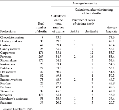
Example 1: The Most Dangerous Profession
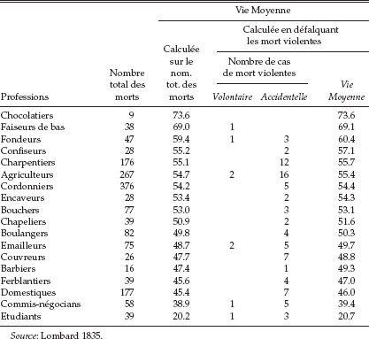
In 1835 the Swiss physician H. C. Lombard published the results of a study on the longevity of various professions. His data were very extensive, consisting of death certificates gathered over more than a half century in Geneva. Each certificate contained the name of the deceased, his profession, and age at death (a sample of Lombard's results translated into English is shown in Table 9.1; the original French is in Table 9.2, in the appendix to this chapter). Lombard used these data to calculate the mean longevity associated with each profession. Lombard's methodology was not original with him, but instead was merely an extension of a study carried out by R. R. Madden that was published two years earlier. Lombard found that the average age of death for the various professions mostly ranged from the early fifties to the midsixties. These were somewhat younger than those found by Madden, but this was expected since Lombard was dealing with ordinary people rather than the “geniuses” in Madden's (the positive correlation between fame and longevity was well known even then). But Lombard's study yielded one surprise; the most dangerous profession—the one with the shortest longevity—was that of “student” with an average age of death of only 20.7! Lombard recognized the reason for this anomaly, but apparently did not connect it to his other results.
TABLE 9.1
Longevity for various professions in Geneva
(from 1776 until 1830)
Example 2: The Twentieth Century Was a Dangerous Time
In 1997, to revisit Lombard's methodology Samuel Palmer gathered 204 birth and death dates from the Princeton (NJ) Cemetery.9 This cemetery opened in the mid-1700s, and has people buried in it born in the early part of that century. Those interred include Grover Cleveland, John Von Neumann, and Kurt Gödel.
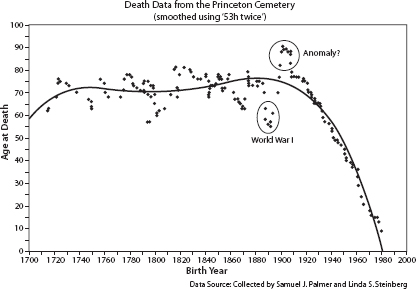
Figure 9.1. The longevities of 204 people buried in Princeton Cemetery shown as a function of the year of their birth. The data points were smoothed using “53h twice” (Tukey 1977), an iterative procedure of running medians.
When age at death was plotted as a function of birth year (after suitable smoothing to make the picture coherent)10 we see the result shown as Figure 9.1. We find that the age of death stays relatively constant until 1920, when the longevity of the people in the cemetery begins to decline rapidly. The average age of death decreases from around seventy years of age in the 1900s to as low as ten in the 1980s. It becomes obvious immediately that there must be a reason for the anomaly in the data (what we might call the “Lombard Surprise”), but what? Was it a war or a plague that caused the rapid decline? Has a neonatal section been added to the cemetery? Was it only opened to poor people after 1920? None of these: the reason for the decline is nonrandom sampling. People cannot be buried in the cemetery if they are not already dead. Relatively few people born in the 1980s are buried in the cemetery and thus no one born in the 1980s who was found in Princeton Cemetery in 1997 could have been older than seventeen.
How can we draw valid inferences from nonrandomly sampled data? The answer is “not easily” and certainly not without risk. The only way to draw inferences is if we have a model for the mechanism by which the data were sampled. Let us consider one well-known example of such a model.
Example 3: Bullet Holes and a Model for Missing Data
The statistician Abraham Wald, in work during World War II was trying to determine where to add extra armor to planes on the basis of the pattern of bullet holes in returning aircraft.11 His conclusion was to determine carefully where returning planes had been shot and put extra armor every place else!
Wald made his discovery by drawing an outline of a plane (crudely shown in Figure 9.2 and then putting a mark on it where a returning aircraft had been shot. Soon the entire plane had been covered with marks except for a few key areas. It was at this point that he interposed a model for the missing data, the planes that did not return. He assumed that planes had been hit more or less uniformly, and hence those aircraft hit in the unmarked places had been unable to return, and thus were the areas that required more armor.
Wald's key insight was his model for the nonresponse. From his observation that planes hit in certain areas were still able to return to base, Wald inferred that the planes that didn't return must have been hit somewhere else. Note that if he used a different model analogous to “those lying within Princeton Cemetery have the same longevity as those without” (i.e., that the planes that returned were hit about the same as those that didn't return), he would have arrived at exactly the opposite (and wrong) conclusion.
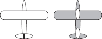
Figure 9.2. A schematic representation of Abraham Wald's ingenious scheme to investigate where to armor aircraft. The left figure shows an outline of a plane, the right shows the same plane after the location of bullet holes was recorded.
To test Wald's model requires heroic efforts. Some of the planes that did not return must be found, and the patterns of bullet holes in them must be recorded. In short, to test the validity of Wald's model for missing data requires that we sample from the unselected population—we must try to get a random sample, even if it is a small one. This strategy remains the basis for the only empirical solution to making inferences from nonrandom samples.
In the cemetery example if we want to get an unbiased estimate of longevities, we might halt our data series at a birth date of 1900. Or we might avoid the bias entirely by looking at longevity as a function of death date rather than birth date.
These three examples are meant to illustrate how far wrong we can go when data that are missing are assumed missing-at-random, that the data that are not observed are just like the data that are observed. Yet this is precisely what is commonly done with value-added models. Can we believe that children who miss exams are just like those who show up? That children who move into or out of the district are the same as those who do neither? There is ample evidence that such assumptions are very far from true.12 It doesn't take much imagination to concoct a plan for gaming the system that would boost a district's scores. For example, during the day of the fall testing have a field trip for high-scoring students; this will mean that the “pre” test scores will be artificially low, as the missing scores will be imputed from the scores that were obtained. Thus when these higher-scoring students show up in the spring for the “post” test, an overlarge gain will be observed. Similarly, one could organize a spring field trip for the students who are expected to do poorly, and hence their “post” scores would be imputed too high. Or do both, for an even bigger boost. Of course sanctions against such shenanigans could be instituted, but clever people, when pressed, can be very inventive, especially when the obstacle to higher ratings for school performance is an unrealistic assumption about the missingness.
It is unknown how sensitive VAM parameter estimates are to missing data that are nonignorable, but ongoing research should have some empirical answers shortly.
I do not mean to suggest that it is impossible to gain useful insights from nonrandomly selected data; only that it is difficult and great care must be taken in drawing inferences. Remember James Thurber's fable of “The Glass in the Field” summarized in chapter 1. Thurber's moral, “He who hesitates is sometimes saved,” is analogous to my main point: that a degree of safety can exist when one makes inferences from nonrandomly selected data, if those inferences are made with caution. Some simple methods are available that help us draw inferences when caution is warranted; they ought to be used.
This chapter is an inappropriate vehicle to discuss these special methods for inference in detail.13 Instead let me describe the general character of any “solution.” First, no one should be deluded and believe that unambiguous inferences can be made from a nonrandom sample. They can't. The magic of statistics cannot create information when there is none. We cannot know for sure the longevity of those who are still alive or the scores for those who didn't take the test. Any inferences that involve such information are doomed to be equivocal. What can we do? One approach is to make up data that might plausibly have come from the unsampled population (i.e., from some hypothesized model for selection) and include them with our sample as if they were real. Then see what inferences we would draw. Next make up some other data and see what inferences are suggested. Continue making up data until all plausible possibilities are covered. When this process is finished, see how stable are the inferences drawn over the entire range of these data imputations. The multiple imputations may not give a good answer, but they can provide an estimate of how sensitive inferences are to the unknown. If this is not done, you have not dealt with possible selection biases—you have only ignored them.
DO TESTS PROVIDE THE EVIDENCE FOR THE INFERENCES VAM WOULD HAVE US MAKE?
If you want to measure change you
should not change the measure.
—Albert Beaton and Rebecca Zwick
The wisdom of Beaton and Zwick's well-known epigram is obvious even to those without extensive psychometric training, yet the validity of most of the inferences from value-added models relies heavily on measures of change based on changing tests and changing constructs. Measuring academic progress is not like measuring height. What constitutes competent reading for a second-grader is quite different from that for a fifth-grader; and it is different in quality as well as general facility.14 This point was elaborated on by Michigan statistician William Schmidt in 2004, when he examined the structure of Michigan's mathematics curriculum from second to eighth grade (summarized in Figure 9.3). Schmidt looked at mathematics because he believed the strong hierarchical structure of the subject meant that it was more likely than other subjects to yield a set of coherent and meaningful change scores. He concluded that it did not; in his words, “Math is not math.”
Schmidt found that the math curriculum's focus in early grades was on the concept and manipulation of numbers; as time went on it shifted, first toward issues in measurement and later toward algebra and geometry. Since sensible tests are aligned with the curriculum, the subject matter of the tests changed over time—even over a year or two. Hence his conclusion that just because you call what is being measured
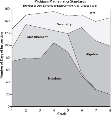
Figure 9.3. The amounts of time that the Michigan math curriculum standards suggest be spent on different components of math from first to eighth grade (from schmidt 2004)
“math” in two different years does not mean that it is the same thing. But how are we to measure change if we insist on changing the measure? What are change scores measuring in such a circumstance?
This is the core question. What is a change score measuring when the construct underlying the measure changes in this fashion? In this instance it is some general underlying ability to do math. By far, the most common analytic result obtained by looking for the best single representation of performance underlying a broad range of cognitive measures is some measure of intelligence—usually called g. This is well described in hundreds of research reports spanning most of the twentieth century.15 We shall not get into the extent to which this kind of ability is genetic, but it is well established that modifying such a derived trait is not easily done, and so it is a poor characteristic by which to weigh the efficacy of schooling. And this is the irony of VAM; by focusing attention on a change score over a multiyear period, VAM directs us away from those aspects of a child's performance that are most likely to inform us about the efficacy of that child's schooling.
The point is surely obvious, but for completeness, let me mention that this kind of value-added assessment is essentially worthless at making comparisons across subjects. It does not tell us how much of a gain in physics is equivalent to some fixed gain in Latin. The same issues that we discussed in earlier chapters are manifested here in spades. But because VAM software gives out numbers, unthinking users can be fooled into thinking that the magic of statistics has been able to answer questions that seem insoluble. It can't.
CONCLUSION
Good teachers understand the wisdom of a Talmudic midrash attributed to Rabban Yohanan ben Zakkai:
If there be a plant in your hand when they say to you, Behold the Messiah!, go and plant the plant, and afterward go out to greet him.
The educational establishment regularly discovers new sources of redemption—this year's promise is that value-added assessment will save us all—but one suspects that the Lord is best served by teachers who find salvation in the routine transactions of their daily work. Value-added assessment may yet help us in this task, but there are many challenges yet to overcome before these models are likely to help us with the very difficult questions VAM was formulated to answer. In this chapter I have chosen what I believe are the three major issues that need much more work:
1. Assessing the causal effect of specific teachers on the changes observed in their students
2. A more realistic treatment of missing data
3. Standardizing and stabilizing the outcome measures used to measure gains.
There are others.
Appendix
TABLE 9.2
Sur la durée de la vie dans diverses professions a Genève
(depuis 1776 á 1830)
This chapter developed from H. Braun and H. Wainer, ”Value-Added Assessment,” in Handbook of Statistics, vol. 27, Psychometrics, ed. C. R. Rao and S. Sinharay (Amsterdam: Elsevier Science, 2007), 867-892.
1 Sanders, Saxton, and Horn 1997.
2 Ballou, Sanders, and Wright 2004.
3 The important model parameter “teacher effect” is misnamed. It represents the variability associated with the classroom, whose value is surely affected by the teacher as well as the extent of crowdedness of the room, the comfort of its furniture and temperature, as well as the makeup of the student body. A fourth-grader with frequent difficulty in bladder control will be disruptive of learning and not under the control of the teacher. A better term would be “classroom effect.”
4 McCaffrey, personal communication, October 13, 2004.
5 The introduction of this section borrows heavily from a 2005 essay written by Paul Holland entitled “Counterfactuals” that he prepared for the Encyclopedia of Statistics in Behavioral Science
6 Random assignment, the usual panacea for problems with diverse populations, does not handle all issues here. Suppose there is a single, very disruptive student. That student is likely to adversely affect the teacher's efficacy. Even if all teachers were equally likely to have that student placed in their class, one of them was unfortunate to get him or her, and hence that teacher's performance will look worse than it ought to without that bit of bad luck. This is but a single example of the possible problems that must be surmounted if student gain scores are to be successfully and fairly used to evaluate teachers.
7 Lord 1967; Holland and Rubin 1983; Wainer 1991; Wainer and Brown 2004.
8 Rubin, Stuart, and Zanutto 2004.
9 Wainer, Palmer, and Bradlow 1998.
10 The points shown in figure 9.1 are those generated by a nonlinear smoothing of the raw data. The smoother used was “53h-twice” (Tukey 1977), which involves taking running medians every 5, then running medians of those every 3, then a weighted linear combination. This smoothed estimate is then subtracted from the original data and the process repeated on the residuals. The resulting two smooths are then added together for the final estimate shown.
11 Mangel and Samaniego 1984; Wald 1980.
12 For example, Dunn, Kadane, and Garrow 2003.
13 For such details the interested reader is referred to Little and Rubin 1987; Rosenbaum 1995; and Wainer 1986 for a beginning.
14 This point was made eloquently by Mark Reckase (2004).
15 The work of Ree and Earles (1991a; 1991b; 1992; 1993), which summarizes a massive amount of work in this area done by military researchers, is but one example; Jensen (1998) provides an encyclopedic description.