Now that you have an understanding of the fundamental Fusion 8 VFX 2D and 3D features, it is time to get into some more advanced 3D effects topics, before I end the book with a chapter discussing how your VFX content can be published across popular devices. Some of the most powerful tools in both 2D and 3D VFX are particle systems, which allow you to control thousands of individual objects acting in concert together to create special effects. Particle systems are powerful as well as advanced, and often involve several areas of physics, which we will cover in Chapter 19, as this is a complex topic that requires two chapters.
In this chapter, we’ll look at how particle systems work, using “emitter ” algorithms that emit and distribute particles, along with particle effects processing algorithms, which then affect each particle’s life , trajectory , scale , opacity , speed , spin , collision , bounce , drag , and similar physical characteristics.
Common Controls: 3D Particle Attributes
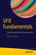
There are some global particle parameters that apply to each particle system (and particle physics ) tool in Fusion 8, and it is logical for us to cover these first, as they clearly represent an overview of many of the core attributes of a particle system, and thus they are a great place to start. Each particle tool will have its own primary Controls tab with the parameters that are unique to that particle tool, as shown circled in red in Figure 18-1. Emitters will have a Region tab and a Style tab , as shown in Figure 18-1, and effects will have a Region tab and a Conditions tab that contains the conditions for applying the particle effect to the particle emitter . We will cover the Effects (Conditions) tab after we cover the Emitter tabs. Before we start a project, we will discuss the particle render node , which is similar in function to the renderer 3D node tool that renders 3D scene components.

Figure 18-1. Four control panel tabs used for particle emitters
Let’s look at the particle Regiontab first, as this tab will allow you to confine the placement of the particle system.
Particle Regions: Where Your Particles Will Exist
Particle regions can be used to restrict a particle tool effect to a 3D (geometric) region or to a 2D (planar) region. It is used to determine the area in which particles will be created using a particle emitter (pEmitter ) node tool. Fusion has seven types of regions, each featuring its own control panel layout, accessed using the Region drop-down selector, shown in the Region tab on the far right side in Figure 18-1. The All region will allow particle to be created everywhere; for 2D mode, the particles will be created anywhere within the boundaries of the image, and in 3D mode this region describes a cubic area.
The Bézier region uses a user-generated polyline to tell the particle emitter where to create the particles. Bézier mode will work in both 2D and 3D particle system modes. Remember that the Bézier polyline region will be created in 2D space. In order to animate over time a shape created using a polyline, or to connect a polyline to another polyline, you’ll need to right-click on the Polyline label, located at the bottom of the control, to select an appropriate option from the polyline context-sensitive menu.
Bitmap dataoutput from one of your 2D tools in the node flow can also be used for a region where particles are emitted.
3D cubic geometrycan also be used to determine a region within which particles are created, as can be seen on the right in Figure 18-1. The height, width, depth, and X, Y, Z positioning can all be determined by a VFX designer and be animated over time.
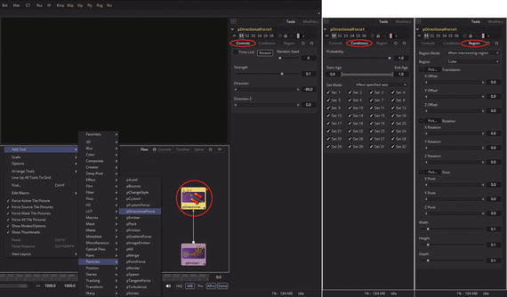
Figure 18-2. Three control panel tabs used for particle effects
3D sphere geometrycan also be used to determine regions in which particles are created, as can be seen on the right in Figure 18-1. The sphere X, Y, Z offset, pivot-point location, and rotation can all be determined by a VFX designer and be animated over time.
The line regio n allows you to determine where a particle or particles should be created. This line should be composed of two endpoints, which can be connected to paths or trackers if necessary. As with the Bézier region, this region type will work in 3D, but the line itself will only be created and adjusted in 2D space.
A 3D mesh region can also be used. In mesh mode, a region can also be restricted by using the Object ID slider. FBX model import with FBX mesh 3D is the norm here, but alembic 3D models (vertex point cloud data) can also be used, with the alembic 3D mesh node tool usage.
The rectangle region is like a cubic region, except that the rectangle region has no depth (that is, no Z coordinates). Unlike other 2D emitter regions, this region could be positioned and rotated in Z space, allowing for some impressive “2D within 3D” visual effects. Next, let’s take a look at particle styles.
Particle Style: Particle Color, Fade, and Lifespan
The particle Style tab can be found in the particle emitter, particle spawn, particle change style, and particle image emitter. In the Style tab, both the type and the appearance of particles are determined. The Style tab provides controls that affect the appearance of your particles, allowing the “look and feel” of particles to be tweaked by a VFX designer. This can even be animated over time.
A Style drop-down menu allows you to define the particle style type, providing settings for different types of particles supported by Fusion’s Particle Tool Suite. Each style type will feature its own specific particle controls, as well as controls that it shares with other style types.
A Point style type is the most commonly used type of particle and produces particles that are one pixel in size; thus, processor power is highly optimized. Controls that are specific to Point style include Apply Mode (blending) and Sub-Pixel Rendered.
Both the Bitmap and Brush style types generate particles based on image data. The Bitmap style type uses image data from another tool in the node flow, and the Brush style type uses TGA (Targa) images that are kept in the Fusion8/Brushes directory.
A Blob style type creates large, soft, spherical particles with Color, Size, Fade Timing, Merge Method, and Noise controls.
The Line style type creates straight-line type particles with an option to set a falloff value. A Size to Velocity control described under Size Controls is often used with the Line type. A Fade control adjusts the amount of falloff spanning the length of your line particle type.
A Point Cluster style type creates small clusters of one-pixel particles. The Point Cluster style is similar to the Point style, and is more memory efficient if large quantities of particles are required. This style type will share controls with the Point style. Additional controls specific to a Point Cluster style type are Number of Points and Number Variance.
The NGon style type is new in Fusion 8, and gives you an NGon generator where you can select the number of polygon sides (hence NGon) and how star-shaped an NGon may be. This is termed NGon Starriness in your Fusion NGon control panel. There are also NGon type presets, including Circular, Circle, NGon Solid, NGon Star, Soft Circular, NGon Shaded In, and NGon Shaded Out.
The Style tab’s Color Controlssection features RGB color controls, which allow you to select RGBA color and alpha values for each of the particles generated by the emitter. You can set a range of colors as well using the Color Variance section, which contains four Low–High dual-range sliders for each RGBA value.
For example, setting a red variance range of -0.2 to +0.2 will produce colors that vary 20 percent on either side of the red channel value set in the color picker just described. To show a color space as 8-bit values (between 0 and 255) or as 16-bit values (between 0 and 65,535), change the values used by Fusion by using the Show Color Aspreference. This can be found in the General tab in the Fusion 8 Preferences dialog .
The “Lock Color Variance” checkbox locks color variance to your particles. Unlocking this allows your color variance to be applied differently across each color channel, yielding a wider range of color variation.
The Color over Life Controlssection contains a standard color gradient widget that allows for a selection of a range of color values. The particles will then conform their coloring to this gradient color-stop collection during their life span.
The left end on a gradient represents the particle color at birth, and the right end shows the color of your particle at death. Additional points that are added to the gradient widget would cause a particle color to shift multiple times throughout its lifespan. This type of control can be used for explosions and other fire-related effects. A gradient widget can be animated over time (right-click on the control and select Animate). The timing for color stops on a gradient will be spline-controlled.
A single Color Over Life spline controlling the speed at which your gradient itself changes can be edited in the spline editor. You could also right-click on your gradient widget and then select a From Image modifier, which will create a gradient from the range of colors in an image specified using a straight line between two points within that image. Pixel colors under that line will form the color gradient color stops.
The Size Controlssection of the Style tab contains size sliders as well as the Size over Lifespline editor graph. The Size and Size Variancesliders are used to specify the size, and the amount of size variation for each particle. Point style doesn’t need size control, as each point is a pixel, and its size is controlled by the pixel pitch (size) of each user’s display.
If the Bitmap particle style is used, a value of 1 indicates that each particle should be exactly the same size as the input bitmap resolution. A value of 2 should scale the particle up in size by 200 percent. For the best particle visual quality, try to make the input bitmap as big as the largest particle produced by the particle system. Remember from the theory Chapter 2 that down sampling by 2X or 4X (or no resizing at 1X) creates the best visual quality.
For a Point Cluster style type, the size control adjusts the density of the cluster, or how close together each particle will get. Essentially, this specifies the size for the cluster.
There are also size sliders that are used to adjust size for the particles based on the velocity or Z depth. The Size to Velocityincreases the particle size relative to a velocity , or speed, of a particle. The velocity of the particle will be added to its size and then scaled by the value of the slider, in case you are wondering how this particular algorithm functions. If a 1.0 is specified using this control, and you have your particle traveling at 0.25, this algorithm will add another 0.25 to your size (Velocity times SizeToVelocity plus Size equals New Size). This control will be used to adjust the size of any style type, but it is the most useful for Line styles.
A Size Z Scaleslider specifies the degree to which a size for each particle would be increased or decreased according to its depth—that is, its position in Z space. The effect of this will be to exaggerate (or reduce) the impact of the perspective. The default value is 1.0, which provides a relatively realistic perspective effect. Objects on the focal plane (Z = 0) would be actual size, and objects farther along Z would become smaller, while objects closer along the Z axis would become larger.
A Size Over Lifespline control graph allows you to draw a spline that determines the size of a particle throughout its life. The vertical scale represents the percentage of the size control, and the horizontal scale represents a percentage of the particle’s life. It is also possible to view and edit the spline graph in the spline editor, just like you did in Chapter 16.
The Fade Controlssection contains a simple range slider that provides a control for fading a particle at the start and at the end of its lifetime using the Fade In– Fade Outdual-range slider widget.
Increasing the Fade In value will cause the particle to fade in at the start of its life. Decreasing the Fade Out value will cause the particle to fade out at the end of its life. The control values represent a percentage of the particle’s overall life; therefore, setting Fade In to 0.1 would cause a particle to fade in over the first 10 percent of its total lifespan.
The Merge Controlssection contains two particle sliders that affect the way individual particles are blended together. The Subtractive–Additive slider allows you to set a blending range from subtractive to additive , and the Burn-In slider will cause particles to over-expose, or become blown out, after they are combined. None of the merge controls will have any effect when used in a 3D particle system, as blending modes are a 2D compositing phenomenon.
The Blur Controls[2D] section of the Style tab contains a set of seven particle controls that would be used to apply a blur to individual particles. Blurring can be applied globally, by age, or by Z-depth position. None of the blur controls would have any effect when used in a 3D particle system.
The Blur [2D]and Blur Variance [2D]sliders will apply blur to each particle independently before these particles are merged together. The Blur Variance slider randomizes the amount of blur applied to each particle to add realism to the VFX. The Blur Over Lifespline graph controls the amount of blur that is applied to a particle over its life. The vertical scale represents the percentage of the blur control, while the horizontal scale represents a percentage of the particle’s life. It’s also possible to view and edit the spline graph in the spline editor, just as you did in Chapter 16.
A Z Blur (DOF)[2D] slider applies blur to each particle based on its position along a z-axis. A DOF FocusRange slider can be used to determine how the degree of focus is calculated for the Z blur. Lower values along Z are closer to the camera, and higher values are farther away. Particles within the range that you set in the DOF Focus Range slider will remain in focus, and particles outside the range will have the blur defined by the Z blur control applied to them.
Different particle style types will have different Apply Modesettings. For example, Point or Point Cluster style types have Add or Merge, which can be applied to 2D particle systems. With Add, the overlapping particles are combined together using a blending algorithm that sums color values for each particle. With Merge, any overlapping particles will be merged together.
The Point or Point Cluster style type “Sub-Pixel Rendered” checkbox determines if a point particle would be rendered using sub-pixel precision, which provides smoother-looking motion but blurrier particles, which will take longer to render.
The Point Cluster style type features a Number of Pointsslider, which determines how many points are in each point cluster, and a Varianceslider, used to randomize this value.
The Bitmap style type has more complex options, including an Animate drop-down widget with options for Over Time, Particle Age, and Particle Birth Time. There are also sliders to set gainas well as time scaleand time offsetdata values. A Brush type also has a Gain slider, used to apply corrections to an overall particle gain, or contrast against the background content (backplate, in our case, Toronto). Note that this parameter can be used with imagery used as a bitmap style or as a brush style. High Gain values produce brighter particle images (or brushes), while a low Gain value will reduce both the brightness and the transparency for the image or the brush.
The Brush type also has a Brush drop-down to select brush images, and a Use Aspect Ratio Fromdrop-down with settings for Image Format, Default Frame Format, and Custom.
The Blob style type has a Noiseslider, which introduces a grain-type noise into the blobby particle system .
The Line style type features a Fade slider, which adjusts the translucency falloff over your line particle’s length. The default value of 100% (1) causes a line to fade out completely by the end of the length.
Particle Sets: Grouping Particles Together
Particle sets allow you to manage individual groups of particles, much like using a material ID to assign different texture map attributes to different faces on a polygonal mesh. The Sets tab is shown in both Figure 18-1 and Figure 18-2, as it has to be available to both emitters (to specify as a set) and effects (to specify what particle sets to process). This allows complex particle systems to be assembled that mix particles together in 3D space or 2D space but allow you to control sets of particles in such a way that they do not affect each other, but rather co-exist together in the same particle physics simulation . We will take a look at using particle sets in the simulation that we create in this chapter and the next, which covers advanced physics. As shown in Figure 18-1, Fusion provides 32 different particle sets that you can utilize to control the configuration of individual particle system dynamics. It’s important to learn how to leverage particle sets, just like it’s important to learn how to leverage material ID for texture map creation and layer grouping for use in digital image compositing pipelines. If you are interested in learning more about image compositing, check out Digital Image Compositing Fundamentals (2015) at www.Apress.com .
Particle Conditions: How Particles Will Be Affected
Particle effects, such as the directional force effect we will be using during this chapter, feature a Conditions tab. This tab contains parameters that specify how that particle effect algorithm will be applied to the particle emitter before it is sent to the particle rendering engine , which we’ll cover next. I added a directional particle node and wired it to the emitter, as shown in Figure 18-2, which opened the particle effect panels, which we’ve covered (controls, sets, and regions), and the Particle Conditions tab, which I’ll cover in this section of the chapter.
A Probabilityslider sets a probability as a percentage chance that the effect will affect a particle. A default value of 100% (1.0) means all the particles will be processed by that effect algorithm. Probability would be calculated for particles on each frame. A particle that is not affected by an effect for one frame has the same chance to be affected in the next frame.
The Start Age– End Agerange slider is used to conform the particle effect being applied to the emitter to a specified percentage of each particle’s lifespan. For example, to restrict the effect to the final third of a particle’s life, set a start value of 0.67 while the end value remains at 1.0. The effect will be processed on frames 67 through 100, or the final third of the particle’s life. The Set Modespecifies how an effect should be applied (all particles or include or exclude the selected set).
Particle Renderer: Making Particle Systems Visible
In order to see particle emitters and effects, you will need to add a pRender node downstream from the other particle nodes, as shown in Figure 18-3. Particle render is where you specify the particle system dimensions, either 3D or 2D—which, as you have seen, affects the usage of blend modes. A pRender tool converts the particle system to either an image (2D) or geometry (3D). The default is a 3D particle system, which must then be connected to a renderer 3D node to produce an image. This allows particles to be integrated with the 3D scene before they are rendered along with the other 3D scene components.

Figure 18-3. Particle rendering menu sequence and control panel
Output modebuttons allow you to select between 3D or 2D output. While the pRender defaults to 3D output, it can be made to render a 2D image sequence. If pRender is not connected to a 3D-only or 2D-only tool, you could also switch it by selecting View ➤ 2D Viewer from its display view context-sensitive menu.
For 3D mode, the only settings in the pRender tool that have an effect include Restart , Pre-Roll , or Automatic Pre-Roll . Sub-frame Calculation Accuracy and Pre-Generate Frames can also be used in 3D mode. All the other settings affect 2D rendering.
The pRender node has a camera input on its node, allowing the connection of a camera 3D node tool. Camera nodes can be used in both 2D and 3D modes to control the viewpoint used to render the output image for your particle system VFX pipeline, just like a real camera controls your view (point).
When a pRender tool is selected and its view dot is set, all the in-view control widgets for particle tools connected to it are seen in the display view. This provides a visual view of the forces being applied to the particle system as a whole.
The Restart and Pre-Roll buttons are used to tell a particle system algorithm the position of each particle on prior frames so that it can calculate the effects of the forces applied to them on the current frame. The controls found here are used to help accommodate this, providing methods for calculating intervening frames. Clicking on the Restart button will restart your particle system at the current frame, removing any particles created up to that point and starting the particle system from scratch at the current frame. Clicking on the Pre-Roll button will cause the particle system to recalculate starting from the beginning of a render range up until the current frame. It will not render the image produced by this calculation; Pre-Roll can only calculate the position for each particle. This provides a way of ensuring that any particle displayed in your viewports will be correctly positioned. If a pRender tool view is on when the Pre-Roll button is clicked, the progress of the pre-roll is seen with particles being shown using point style to save on system-processing overhead.
The Automatic Pre-Roll selection tells a particle system to automatically pre-roll particle calculations to support your current frame whenever the current frame changes. This prevents your needing to manually click the Pre-Roll button whenever advancing through time in increments larger than one frame. This progress of a particle system during automatic pre-roll is not displayed in your pRender view so as to prevent visual workflow interruptions.
There are post-render output settings for applying blur, glow, and blur blend as well as settings for integration method, subframe calculation accuracy, and pre-generating frames. There are options to kill particles that leave your view, death merge particles, and to generate a Z buffer for your particle system. The Blur, Glow, and Blur Blendsliders apply Gaussian blur , glow, and blending to the 2D particle system image as it is rendered.
This can be used to soften 2D particles or to blend them together. Your result is the same as adding a blur node after a pRender tool in the flow node editor.
The Sub-Frame Calculation Accuracy slider will specify a number of sub-samples taken between frames when calculating the particle system. High values will increase the accuracy of your particle-system algorithm’s calculations and will increase the length of time that it will take to render the particle system.
The Pre-Generate Frames slider tells the particle system to pre-generate a specified number of frames before your first frame. It is used to give your particle system an initial state from which to start calculating its particle system algorithms.
Clicking the “Kill particles that leave the view” checkbox would kill all particles that leave the visible boundary for a 2D image. This can be used to speed up render time. Particles destroyed with this option will not return, so make sure this is what you want to do for your VFX particle simulation objectives.
Selecting the “Generate Z Buffer” checkbox will cause the pRender tool to produce a Z buffer channel for your image. The depth of each particle is represented in the Z buffer. This auxiliary channel can then be used for 2D depth-compositing operations like depth blur, depth fog, or downstream Z merging. This option increases rendering time for a particle system, as you probably surmised.
Clicking the “Depth Merge Particles” option causes the particles to be merged together using depth-merging algorithms rather than using layer-centric blending techniques.
Particle System Project: Adding Core Nodes
Assuming you have followed Figures 18-1 through 18-3 and added pEmitter, pDirectionalForce, and pRender nodes using the Add Tool ➤ Particles context menu, let’s add an image next that we can composite the particle system over, since many times that is what you are going to want to do for a VFX project pipeline. I used pexels.comto find a nice, free for commercial use image of the Toronto skyline taken by photographer Amarpreet Kaur . I used an image loader to load this into my project and an image saver to save out the particle system animation. We will add in other nodes as we create this project over the next couple of chapters. Figure 18-4 shows the image I chose on pexels.com by clicking on it. We can use Fusion tools to adjust this image as needed to fit our particle system animation, adding nodes into our VFX pipeline as we go. This is one of the most impressive aspects of Fusion 8’s visual-programming paradigm—being able to build and refine a VFX project, and its visual results, by adding new nodes and wiring them together.
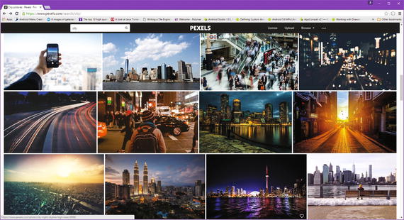
Figure 18-4. Go to pexels.com and find a good image to use as a background plate
Click on the HD image you want to use, and download it to your project folder; in my case, this was VFX_Fundamentals. The work process I used is shown in Figure 18-5, on the right side.
Figure 18-5. Download a royalty-free, HD, high-resolution image
Next use Add Tool ➤ Composition ➤ Merge to add a node so as to composite your particle system’s foreground over your cityscape background. Wire the cityscape loader into the merge node, wire the merge output into a CityScape.MP4 saver, and wire a pRender output into the Merge1.Foreground input, as seen in Figure 18-6.
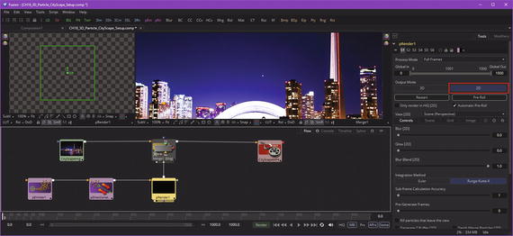
Figure 18-6. Add an image loader, image saver, and a merge node
Next, set a Number value of 1 (also pick a Random Seed). I started out with Lifespanat 50 and a Velocity of 0.15. I set an Angle value of 90° and an Angle Varianceand Z Varianceof 10°, as shown on the right in Figure 18-7, highlighted in red.

Figure 18-7. Specify the starting pEmitter particle control settings
Next, select your Region tab, and select Line from the Region drop-down menu, as shown in red in Figure 18-8.
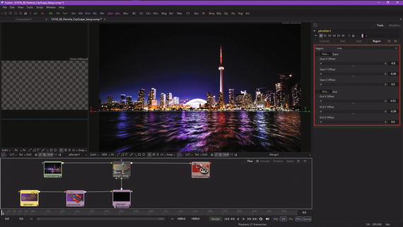
Figure 18-8. Specify the line emitter region, and place it on the Toronto City Waterfront (beach)
Place the line right on the Toronto waterline, or beachfront, as shown by widgets on the left and right side of the image in Figure 18-8. I set a particle type of Brush in the Style tab, shown in Figure 18-9, so I could see particle trajectories and placement, as points were too small (due to sub-pixel rendering) on this 2400 x 1600 image.
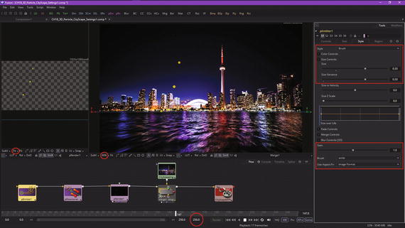
Figure 18-9. Specify the Brush particle style so that you can tweak its parameters
You may have noticed in Figures 18-8 and 18-9 that there is a resolution disparity between our 2400 x 1600 image and the particles’ rendering view, which is labeled with an HDTV 1920 x 1080 resolution. Clearly, our particle canvas must match up with our image. I’m getting imprecise results as I play the particle system, and other than my as yet unrefined settings, this would be the most significant reason for that. Select the pRender node, as is seen in Figure 18-10, and conform the width and height to the 2400 x 1600 image. You will see that you have to readjust your Line emitter, which is why the particles were not emitting correctly relative to the backplate image. Once you do this, the pRender preview and merge View2 will match up, the particles will correctly emit from the line emitter placed along the Toronto beachfront, and we are now ready to continue.

Figure 18-10. Synchronize the resolution for the pRender node tile to match backplate image
We’ll still need to tweak settings during the entire VFX pipeline creation process, but let’s take a look at your pSpawn node, so we can add a trail of sparks from the primary particle.
Particle Spawn: Particles Birthing Other Particles
The particle spawn or pSpawn tool can turn each of your particles into its own parent emitter, allowing a particle to produce child particles of its own, which is why it is called Particle Spawn. The original particle will continue to exist until the end of its lifespan, and each of the child particles that it emits (spawns) during its lifespan becomes wholly independent, with its own lifespan, and its own particle characteristics, which we are covering during this chapter.
As long as a particle is processed by a pSpawn algorithm, it can continue to generate child particles. Be sure to conform the settings for this tool to limit particle generation, as new particles generated must then be managed by the particle system, using your valuable CPU power. Settings that can limit runaway child particles include start or end age, probability, sets and regions, and pEmitter parameter animation, so that particles are in play and being operated on by the CPU only when necessary.
Right-click in the flow node editor and use an Add Tool ➤ Particles ➤ pSpawn menu sequence to add a particle spawn node to your project, as is shown in Figure 18-11. Also make sure an end range has been set in the time ruler. I set 250 (as seen in Figure 18-9) as my particle system duration, at least for now.
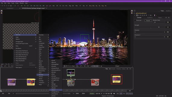
Figure 18-11. Add a pSpawn node, using Add Tool ➤ Particles ➤ pSpawn
This pSpawn tool has a significant number of parameters, most of which mirror parameters in the pEmitter tool. pSpawn is both an emitter and an effect and, as such, has tabs for Controls, Sets, Style, Conditions, and Region. There are several parameters unique to this pSpawn tool. Let’s discuss the new parameters first, before we set our initial parameters.
The “Affect Spawned Particles” checkbox, when selected, will cause particles created by this spawn algorithm to become seeds for the spawn tool on subsequent frames. This can exponentially increase the number of particles in the particle system on each subsequent frame of your particle system timeline (mine is 250) and can therefore affect render time significantly. This option should only be used when absolutely necessary in a VFX project.
The Velocity Transferslider specifies how much velocity from the parent particle will transfer to the child particles that it spawns. The default value of 1 causes each new particle to adopt 100 percent velocity and direction from the parent particle. Lower velocity transfer data values should transfer less of the original parent particle’s motion attributes to child particles and therefore a value of (or near) zero will create independent child particles, with a mind of their own (if we adhere to the parent-child paradigm we are using here).
Let’s set our Number of (Spawn) Particles to 5 and Angle and Angle Variance to 360°. I used Velocity of .002 and Velocity Transfer of 0.03 so that the parent particle leaves a trail of child particles. As you can see in Figure 18-12, this is working well, but my parent particles are still leaving the screen, so my Gravityparticle effect parameter is still not set properly. As you can see, creating a particle simulation is a refinement process.
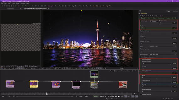
Figure 18-12. Set pSpawn parameters for Number, Angle, and Velocity
Figure 18-13 shows the areas that I looked at to get the gravity, which is provided by a -90° directional force, to work properly. First, I set a longer particle lifespan and variation, to see if the particles would start to fall. They didn’t. I next set the Region for this pDirectionalForce to affect all of the particles in the simulation. That did not work either! So I looked at the pEmitter Sets tab, finding that I hadn’t assigned any particle set to these particles! After I selected Set 1, my gravity worked perfectly, and I was ready to proceed in working on the VFX project. It is best to perfect portions of the pipeline before adding more complexity, which is the work process I am using during this book.
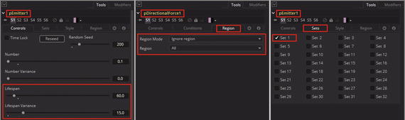
Figure 18-13. Tweaking the settings to get the particle gravity to work optimally
Since Spawn is an effect as well as an emitter, let’s set the Spawn Sets tab to only affect these Set 1 particles. Now we are ready to add more characteristics to the particle system. I want to show you how to create exploding effects, so let’s add a second pSpawn node to do this. Wire your pSpawn2 in between the pSpawn1 and pDirectionalForce1 nodes, and set your Number to 250, Variance to 10%, Lifespan to 40, and Lifespan Varianceto 20%. In your Velocity section, set Velocity Transferto zero, Velocity to 0.125, Velocity Varianceto 5%, Angle and Angle Z to 0, and Angle Varianceand Angle Z Varianceto 360°. Leave the Region set to Affect All Regions.
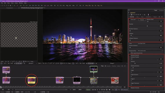
Figure 18-14. Add a second particle spawn node and set the parameters
Next, let’s configure your Set and Condition parameters!
As you can see in Figure 18-15, we are going to set this second particle spawn algorithm to label its particles as Set 2 so that we can apply different physics attributes, which we are going to be covering during the next chapter, to the explosion and not affect the particle trail created by the first particle spawn algorithm. This is done by using the Sets tab, seen on the left side of Figure 18-15. We also want this explosion to occur when the parent particle dies, or just before it does, at a 99% of lifespan point in time, which is shown in the Conditions tab and set using the Start Age slider. We also want to use the Set Mode of Affect specified sets and then set the Set 1 as the set to be affected, as is shown on the right side in Figure 18-15.
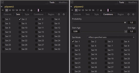
Figure 18-15. Set as Particle Set 2 and set to Affect Particle Set 1
Notice that if we change particle system parameters requiring lots of algorithmic processing, the pRender tile turns into the progress bar for particle processing upstream of it, as shown circled in red in Figure 18-16. Now we are ready to tweak our pSpawn2 settings to refine this explosion effect, before we finish up with this chapter.
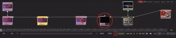
Figure 18-16. pRender node tile preview progress bar shows particle system processing
Now we have a nice, complex particle system simulation that uses only one primary emitter to create hundreds of sparks, particle trails, and particle explosions, all affected by gravity. We will be covering other physics algorithms in the next chapter. This pDirectionalForce algorithm can be used to simulate many physical systems other than gravity, so I am covering this topic in this chapter, since we have a lot more to cover in Chapter 19. As you see in Figure 18-17, your happy face placeholder particles are shooting up and falling back and then exploding as intended, and all we have to do is reduce the number of particles used, and refine some of the variation parameters to get more realism into the particle simulation. I will always try to reduce the number of particles used as much as possible, while still getting the desired visual effect, for data footprint and CPU optimization reasons.
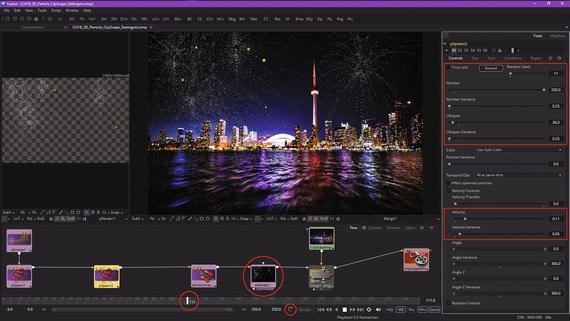
Figure 18-17. Explosions can be seen rendering in the pRender node, View1, and View2
Before we finish up with the chapter, let’s take a break from particle systems and add a node or two on the imaging side of our VFX pipeline, to better optimize the background image quality, so as to have good contrast for use with the particle system simulation.
Background Plate Optimization: ColorCorrector Node
I’m going to use a color correctionalgorithm to darken the sky and brighten the lights in the buildings and their reflections on the water. I’m thinking of refining the particle system into a fireworks simulation, and sparks look better in front of a darker sky.
As you can see in Figure 18-18, I have added an Add Tool ➤ Color ➤ Color Correctornode, and wired it between the loader and merge nodes, reconfiguring the node tile flow during the process. We have created an incredibly robust VFX project using only nine nodes here in Fusion 8!

Figure 18-18. Darken the sky and brighten the color reflections in the backplate using a ColorCorrector Node
I pulled the middle tones 0.8 to the right to darken the sky, and I pulled the highlights to the left 0.7 to saturate the color reflections on the water, as you can see in Figure 18-18.
I wanted to set up this pipeline now so I could tweak it more later, when the particle system work is complete, and it can be used as a visual reference against what I am doing with this ColorCorrector1 node. That is what is great about how you build your VFX processing pipeline in Fusion 8 using node tool tiles, as you have fine-tuned control over your pipeline, the VFX project it creates, and how the assets and intermediary assets (things like masks and geometry) are displayed in Fusion.
Summary
In this eighteenth chapter, we took a look at particle system dynamics, concepts, forces, emitters, sets, regions, settings, and rendering. We looked at all of the various parameters used to set up emitters and effects, how to render particle systems and composite them over imagery, and how to use sets to combine multiple particle systems seamlessly as if they were one particle system simulation. We looked at different types of emitters and used a brush emitter as a proxy to refine settings. We also got some more practice with digital image adjustment. In Chapter 19, we will look at particle system physics.