
Chapter 10
Hierarchy
Hierarchy should be used extensively in a design to divide-and-conquer the design problem. Furthermore, third-party components can be incorporated into a design more easily this way and this leads to a higher degree of confidence in the integrity of the design.
The natural form of hierarchy in VHDL, at least when it is used for RTL design, is the component. Do not be tempted to use subprograms as a form of hierarchical design! Any entity/architecture pair can be used as a component in a higher-level architecture. Thus, complex circuits can be built up in stages from lower-level components.
It is possible to design parameterised circuits using generics. The combination of generics with synthesis, which allows the design of technology-independent circuits, is a very powerful combination.
There are a number of reasons for using hierarchy.
Each subcomponent can be designed and tested in isolation before being incorporated into the higher levels of the design. This testing of intermediate levels is much simpler than system testing and consequently is usually more thorough. Using components for hierarchy is compatible with the Test-Driven Design paradigm since it makes testing of subsystems easier. This means that the designer can have a high degree of confidence in the subcomponents and this also contributes to the overall integrity of the design.
It is good practice to collect useful subcomponents together into reusable libraries so that they can be used elsewhere in the same design and later on in other designs. One of the great gains of logic synthesis is that such modules are technology independent and so can be reused in a wide variety of different projects. This means that, over a period of time, the level of reuse in each design increases as more components become available.
It is important to have a strategy to collect useful components together into libraries for reuse. Many reuse policies, both in software and hardware design, fail due to excessive bureaucracy, which discourages users from submitting reusable components to be added to the library. A realistic reuse policy should therefore be based on the minimum of bureaucracy to encourage the generation and use of such components.
The first official version of VHDL, VHDL-1987, was very clumsy in its handling of components. The original language designers concentrated on making the component mechanism as flexible as possible, and succeeded in this aim, but the result was cumbersome in use and the full flexibility was rarely used. This form of component is known as “indirect binding”. A simpler form of components was added in VHDL-1993 to make them more usable. This form of component is known as “direct binding”.
The use of components will be illustrated first with a complete example using indirect binding. Then, this example will be converted to use the simpler direct binding. Direct binding is the form that will then be used throughout the rest of the book – indirect binding is included for completeness.
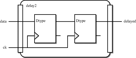
The example is a trivial one so that the focus is on the components rather than their contents. It is a simple two-register pipeline. The problem is illustrated by Figure 10.1, and is to create a circuit containing two register components connected in series.
Figure 10.1 Target circuit.
It will be assumed that the register component that will be used already exists and has the following interface:
library ieee;
use ieee.std_logic_1164.all;
entity Dtype is
port (D, Ck : in std_logic; Q, Qbar : out std_logic);
end;
Due to the flexibility of the indirect binding mechanism in VHDL, there is more than one way that this could be described using components, depending on the level of detail that is given. Some of the information required to create component instances is optional and, if omitted, default values will be used. This is covered in detail in the following subsections. The target circuit in its fullest form is:
library ieee;
use ieee.std_logic_1164.all;
entity delay2 is
port (data, ck : in std_logic; delayed : out std_logic);
end;
architecture behaviour of delay2 is
-- component declaration
component dtype
port (d, ck : in std_logic; q, qbar : out std_logic);
end component;
-- configuration specification
for all : dtype use entity work.Dtype(behaviour)
port map (D => d, Ck => ck, Q => q, Qbar => qbar);
signal internal : std_logic;
begin
-- component instances
d1 : dtype
port map (d => data, ck => ck, q => internal, qbar => open);
d2 : dtype
port map (d => internal, ck => ck, q => delayed, qbar => open);
end;
Note that the entity has just three port declarations, since the target circuit only has a delayed output, compared with the dtype component that has both q and qbar outputs.
The architecture has been called behaviour, despite the fact that it contains no behavioural VHDL, because it is part of a synthesisable design. The architecture name should reflect the usage of the architecture, not its contents.
The architecture contains three sections related to the use of components. These have been labelled with comments giving the names of the three parts: component declaration, configuration specification and component instance. It is the component instances that make up the circuit. The component declaration and configuration specification are declarations that control the selection and means of connection of the component instances.
The following three subsections will discuss the three parts of this architecture.
10.2.1 Component Instances
Component instances are concurrent statements. In this sense, they model hardware components closely, because hardware is inherently concurrent.
In the above example, there are two component instances, which have been labelled d1 and d2. These labels are for reference only but must be present and must be unique within the architecture. Each component instance in this example creates a subcircuit using the component dtype and the connections to this component.
It should be noted that the component instance is an instance of the component declaration and not the entity. The relationship between the component declaration and the entity is controlled by the configuration specification.
In the example, the distinction between the entity and the component declaration has been made by giving the entity initial capitals on its name and the name of its ports. The component instance and the internal signals in the target circuit have been given lowercase names. Put another way, everything declared within the target circuit has lowercase names, whereas everything outside the target circuit – namely the entity being used as a component – have initial capitals. This distinction is made just for clarity and is not of any other significance, since VHDL is not sensitive to the case of names anyway.
The component instance part of the example is reproduced here:
d1 : dtype
port map (d => data, ck => clock, q => intern, qbar => open);
d2 : dtype
port map (d => intern, ck => clock, q => delayed, qbar => open);
A component instance has two parts, the component name and its port map. The component name part is fairly self-explanatory – it labels the instance (in this case d1) and then gives the name of the component that is to be used for the instance (in this case dtype). Note that this is the name of a component declaration, not the entity. This component must be declared before it can be instanced, either in the architecture (see later) or in a package (see Section 10.4).
The port map describes how signals in the architecture are to be connected to the ports of the component. There are two ways of specifying the port map: using named association or positional association. The form shown is named association.
With named association, each port is listed by name (remember that these are the component ports, not the entity ports). The port name is then followed by the "=>" symbol, known as finger and pronounced ‘connected to’ and then the signal that it is to be connected to. This signal must, of course, be declared as either a signal in the architecture or a port in the entity of the target circuit. Output ports on the component can be left unconnected by using the keyword open.
With positional association, the port names and fingers are omitted, and the signals are listed in the same order as the port declarations in the component. Thus, the above example could be rewritten using positional association:
d1 : dtype port map (data, clock, internal, open);
d2 : dtype port map (internal, clock, delayed, open);
Positional association is clearly simpler and shorter, but named association has the advantage of acting as a reminder of which port each signal is being connected to. This means that the component instance is more self-explanatory to a reader of the model. With named association it is also possible to change the ordering of the ports if a different ordering seems more natural to show the data flow in the design. Finally, the named association gives a VHDL analyser an extra opportunity for checking the consistency of the design.
10.2.2 Component Declarations
The component declaration defines a component that can then be instanced. It is in effect saying that, somewhere, there is an entity that can be used as a component. However, the component declaration itself does not specify where that entity is or even what it is called or what its ports are called. This is the job of the configuration specification, which is described in the next section.
In practice, the component declaration usually matches the entity that it represents exactly. That is, the name and the port names and their order are taken directly from the entity. The only difference is that the component has a slightly different syntax. In the following two examples, the entity and its representative component are shown with their differences underlined.
The entity for the Dtype was declared as:
entity Dtype is
port (D, Ck : in std_logic; Q, Qbar : out std_logic);
end;
The component dtype is declared as:
component dtype
port (d, ck : in std_logic; q, qbar : out std_logic);
end component;
The need for a component declaration is probably the clumsiest part of the use of indirect binding. However, the need for components declarations can be reduced by using component packages. There is no need for component declarations at all when using direct binding.
10.2.3 Configuration Specifications
The configuration specification closes the gap between entities and their component declarations. The reason for separating the entity and its components is a feature of the language that allows the association (technically known as binding) between component and entity to be made as late as possible in the simulation process. In fact, binding is not carried out during the analysis phase at all, it is deferred until elaboration – the start of simulation. This means that a hierarchical design can be compiled in any order – with the extreme cases being top-down or bottom-up.
The configuration specification defines where the entity is to be found, what it is called and how the component ports relate to the entity ports. The full form of a configuration specification is long-winded, but all aspects of it have sensible defaults and indeed, the configuration specification is itself optional and can be omitted completely to get all the default options.
First, an explanation of the parts of a configuration specification. The configuration from the example is reproduced here:
for all : dtype use entity work.Dtype(behaviour)
port map (D => d, Ck => ck, Q => q, Qbar => qbar);
The configuration specification has three parts.
The first part specifies the components that the configuration applies to. In this case, the components are selected by the keyword all, so all the components called dtype are configured by this specification. It would have been possible to have separate configuration specifications for each component separately:
for d1 : dtype ...
for d2 : dtype ...
The second part of the configuration selects the entity to use for the component. This is known as the entity binding. The entity binding must specify which library the entity is in as well as its name. In this case, the entity is specified as being in the same library as the target circuit, so is referred to by the reserved library name work.
The entity binding also specifies an architecture to use for the component. Multiple architectures are rarely used in RTL design, so the ability to select an architecture is rarely needed. In the example, the architecture behaviour is specified. To omit the architecture, omit the parentheses as well. The default architecture is, strangely, the most recently compiled one! For single-architecture entities, though, this means that the only architecture present is automatically selected.
There are other forms of binding, but these are not generally supported by synthesisers so will not be covered here.
The third part of the configuration specification defines the port bindings. That is, it associates the entity ports with the component ports. This allows port names to be different in the entity and the component, although it is hard to imagine any reason for doing this.
The port binding is optional, and if omitted, the component ports are bound to entity ports of the same name. If present, then the port binding, enclosed in parentheses, is a list of entity ports associated with their corresponding component ports. In other words, each entry in the port binding is the entity port name, finger, then the component port name. The entity port name and finger can be omitted, in which case the component ports are bound to the entity in the order defined on the entity.
10.2.4 Default Binding
If the configuration specification is missing completely, then the component is bound to an entity of the same name as the component, in the work library, and to the architecture most recently analysed, and the ports are bound to the entity ports with the same names. Since this is the most commonly desired binding, configuration specifications would appear to be unnecessary.
However, there is one case where configuration specifications are necessary. This is where the component is to be bound to an entity in a different library. Also, some VHDL systems do not implement the default entity binding, so some form of configuration declaration must be included even with an entity in library work. These systems do not implement default entity binding because, so the vendors argue, the VHDL standard does not require it. This is a moot point and default binding has become the accepted practice, so these vendors are out of line with most users' expectations.
Binding could be achieved by making all of the entities in the library visible with a library and use clause. For example, if the component was in a library called basic_gates, then the following library and use clauses could be added to the architecture to make all the entities in that library visible, making a configuration specification unnecessary:
library basic_gates;
use basic_gates.all;
architecture behaviour of delay2 is
component dtype
port (d, ck : in std_logic; q, qbar : out std_logic);
end component;
signal internal : std_logic;
begin
d1 : dtype port map (data, clock, internal, open);
d2 : dtype port map (internal, clock, delayed, open);
end;
The problem with this approach is that all the entities in that library become visible, regardless of whether they are going to be used, causing what is known as clutter in the number of names visible at once. This could result in name clashes, especially if more than one library is made visible in this way. A better approach that avoids clutter is to use the minimum configuration specification, which just binds the entity and uses the defaults for everything else:
library basic_gates;
architecture behaviour of delay2 is
component dtype
port (d, ck : in std_logic; q, qbar : out std_logic);
end component;
for all : dtype use entity basic_gates.Dtype;
signal intern : std_logic;
begin
d1 : dtype port map (data, clock, intern, open);
d2 : dtype port map (intern, clock, delayed, open);
end;
Note that the library clause is still needed in order to be able to make the entity binding.
Due to the difference in interpretation of the default binding rules of VHDL, it is recommended that at least a minimum configuration is used, even for creating components of entities that are in library work; don't rely on the default entity binding.
10.2.5 Summary of Indirect Binding Process
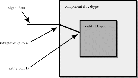
The best way to think of the relationship between a component instance, the component declaration and the entity being used as a component is as a two-layer binding process.
The outer layer defines the connections between the signals in the target circuit and the ports of the component and is described by the component instance.
The inner layer defines the binding between the component and the entity and is described by the configuration specification.
This two-layer model is illustrated by Figure 10.2.
Figure 10.2 The two layers of indirect binding.
A simpler form of component instantiation is direct binding. In direct binding, the component instance is directly bound to the entity without the need for an intermediate component declaration or a configuration specification. Another way of putting this is that direct binding has only one layer, unlike the two layers of indirect binding.
The syntax of direct binding is like a combination of the component instance and the configuration specification. This allows the above example to be reduced to a very simple architecture indeed:
library basic_gates;
architecture behaviour of delay2 is
signal internal : std_logic;
begin
d1 : entity basic_gates.dtype(behaviour)
port map (data, clock, internal, open);
d2 : entity basic_gates.dtype(behaviour)
port map (internal, clock, delayed, open);
end;
Direct binding is the recommended form for simple hierarchy within a design. However, indirect binding does have its uses as the next section shows.
It can be convenient to collect together a set of components within a project or a component library and write a package containing all of their component declarations in one place. This package can then be used to instantiate those components and, because it is in one place, act as a user reference as well. It is good practice to do this if you are responsible for a reusable component library for example. This approach makes use of indirect binding with the component declaration moved into a separate package.
Once you have such a package, it is only necessary to have a use clause for the package to make use of the component. Note that this is only worthwhile for commonly used components, since it is still necessary to write the component declaration once – in the package! For simple hierarchy within a design, use direct binding.
To illustrate the use of component packages, the previous indirect binding example will be used. The package containing the component declaration would look like:
package basic_gates is
component dtype
port (d, ck : in bit; q, qbar : out bit);
end component;
... other components
end;
Only the component declaration can be placed in a package; the configuration specification is part of the binding process and so must be part of the specific design, by placing it in the architecture where the binding is to take place.
Assuming that this package is analysed into the current work library, the component would be used in the target circuit as follows:
use work.basic_gates.all;
architecture behaviour of delay2 is
signal intern : std_logic;
for all : dtype use entity work.Dtype;
begin
d1 : dtype port map (data, clock, intern, open);
d2 : dtype port map (intern, clock, delayed, open);
end;
This example uses indirect binding with the minimum configuration specification, as recommended in Section 10.2.
The package can be analysed into any library in this way. It need not be in the same library as the entity that its component declarations represent. However, it is good practice to analyse the package into the same library as the entities. Such component packages are quite commonplace, especially for reusable libraries. These libraries contain whole families of related circuits described as entity/architecture pairs. Then, all the entities are declared as component declarations in a single package for ease of use. Often, the package is given the same name as the library to make its purpose clear.
If the entities are in a different VHDL library from your design, then a configuration specification is always required. Taking the same example as before, and again assuming that the Dtype entity and its component package are in the library basic_gates rather than work, the architecture now looks like:
library basic_gates;
use basic_gates.basic_gates.all;
architecture behaviour of delay2 is
signal intern : bit;
for all : dtype use entity basic_gates.Dtype;
begin
d1 : dtype port map (data, clock, intern, open);
d2 : dtype port map (intern, clock, delayed, open);
end;
It is possible to design parameterised circuits using generics. The combination of generics with synthesis, which allows the design of technology-independent circuits, is a very powerful combination. Generics are especially powerful where there is an established reuse policy, so useful models are written in a generic style with reuse in mind. Indeed, it is good practice to consider the reusability of subcomponents of a design during the early stages of the design cycle, possibly as a part of the design review process, so that subcomponents recognised as reusable are earmarked for parameterisation.
Probably the most common use of generics is to parameterise the port width of a component, so the same ALU model, for example, can be used as an 8-bit ALU in one design and then as a 16-bit ALU in another design. Other uses are to parameterise the number of pipeline stages in a design or to include/exclude features such as output registers.
10.5.1 Generic Entity
To illustrate the use of generics, a simple example will be used. The example is a shifter with a parallel load. Once again, this example does not really represent typical usage since such a simple circuit would be embedded in a bigger design and not have an entity and architecture of its own. A simple example is used so that the focus of attention is on the VHDL, not the circuit.
The interface of the shifter is:
library ieee;
use ieee.std_logic_1164.all;
entity shifter is
generic (n : natural);
port (ck : in std_logic;
load : in std_logic;
shift : in std_logic;
input : in std_logic_vector(n-1 downto 0);
output : out std_logic);
end;
This entity has an extra field – the generic clause – that defines the circuit's parameters. In this case, there is just one parameter, n, which specifies the width of the shifter. This has then been used to define the width of the input port. Simple calculations can be used in the definition of port widths, provided they can be evaluated as a constant value once the generic parameter is set to an actual value. Generally, this restricts you to using built-in operators on integer, as in this case where the range of an n-bit signal is defined as (n-1 downto 0), which uses built-in integer subtraction.
Before going into the writing of a generic model, the way in which this entity would be used as a component will be illustrated.
10.5.2 Using Generic Components
A generic entity is used as a component in the same way as a non-generic entity. The only difference is that a value must be specified for the generic parameter for each instance of the component. This value must be a constant so that the synthesiser can calculate the size of the ports and is usually given directly as a numeric value in the component instance's generic map.
For example, to use the shifter parameterisable entity to make an 8-bit shifter component, the following would be used:
library ieee;
use ieee.std_logic_1164.all;
entity shifter8 is
port (ck : in std_logic;
load : in std_logic;
shift : in std_logic;
input : in std_logic_vector(7 downto 0);
output : out std_logic);
end;
architecture behaviour of shifter8 is
begin
shift : entity work.shifter
generic map (n => 8)
port map (ck, load, shift, input, output);
end;
The component instance contains an extra field – the generic map – which gives the value to be used for the generic parameter. This instance of the shifter circuit will be built with this value substituted throughout in place of the parameter n.
The generic map can alternatively be written using positional association:
shift : entity work.shifter
generic map (8)
port map (ck, load, shift, input, output);
The rule in synthesis, remember, is that all signals must be of a known size for the synthesiser to be able to calculate the size of the bus to implement. With parameterised circuits, this calculation is carried out after generic parameters have been replaced with their actual values. Therefore, a generic can be treated as a constant value.
In the original entity definition the port input was defined as:
input : in std_logic_vector(n-1 downto 0);
When an instance is created, the value n will be replaced by its actual value. In the example above, the value 8 was used. This means that the port declaration becomes:
input : in std_logic_vector(7 downto 0);
So the synthesiser creates an 8-bit bus for this port.
10.5.3 Parameterised Architecture
Now that the use of a generic entity as a component has been discussed, it is time to get down to actually writing the generic circuit.
Within an architecture, a generic parameter acts as if it was a constant value, so can be used wherever a constant value would be used.
The architecture for the ripple carry adder is:
architecture behaviour of shifter is
signal store : std_logic_vector(n-1 downto 0);
begin
process
begin
wait until rising_edge(ck);
if load = '1' then
store <= input;
elsif shift = '1' then
store <= store(store'left-1 downto 0) & store(store'left);
end if;
end;
output <= store(store'left);
end;
Note how the store signal that is then registered by the register process is defined in terms of the generic parameter n. Then, within the architecture, the bounds of this store are referred to using attributes rather than constant values, so that they can adjust to stores of different sizes. For example, the shift is implemented using a slice of the store:
store <= store(store'left-1 downto 0) & store(store'left);
The rule with slices is their bounds must be constant to be synthesisable. In this case, this will evaluate to a constant once the attribute has been substituted. For the case where n = 8, the store has a range of (7 downto 0):
store <= store(7-1 downto 0) & store(7);
This is now expressed in terms of built-in integer operators and can be evaluated as a constant slice, concatenated with a single bit to give a result that is the same size as the store:
store <= store(6 downto 0) & store(7);
This could alternatively have been written in terms of the generic parameter instead:
architecture behaviour of shifter is
signal store : std_logic_vector(n-1 downto 0);
begin
process
begin
wait until rising_edge(ck);
if load = '1' then
store <= input;
elsif shift = '1' then
store <= store(n-2 downto 0)
end if;
end;
output <= store(n-1);
end;
Again, all slices and indices are expressed as calculations involving integer and its built-in operations, so this generic architecture is synthesisable.
10.5.4 Generic Parameter Types
In simulation VHDL, generic parameters can be of any type. However, synthesisers are limited in the types of generic parameter supported. The only types that can generally be used are integer types, although some synthesisers also allow enumeration types, of which the most useful are probably boolean, bit and std_logic.
The shifter circuit conformed to these restrictions, since the generic parameter type was natural, a subtype of integer. The use of subtype natural tells users not to try to create a shifter with a negative number of bits.
All the bit-array types used for synthesis are indexed by integer. This is true of bit_vector, std_logic_vector and the signed, unsigned, sfixed, ufixed and float synthesisable types. Therefore, integer generics can be used to constrain array ports of any of these types.
Generic parameters of other types can make other features parameterisable. For example, type boolean can be used to specify conditional features. An example of this will be deferred until Section 10.6, because conditional features are most easily described using if generate statements which are covered in that section.
Generate statements are used to create replicated or conditional hardware structures. Generate statements are concurrent statements that can be used in any architecture, but they are described here because they really come into their own when used with generics in parameterised circuits.
There are two types of generate statement: the for generate statement for replicated structures and the if generate statement for conditional structures.
10.6.1 For Generate Statements
The for generate statement replicates (copies) its contents a specified number of times. It is in effect a concurrent form of for loop. However, being a concurrent statement, it can be used to replicate any other concurrent statements, including processes, concurrent signal assignments, component instances and other generate statements. This means that for generate statements can replicate structures that are impossible to replicate using for loops. The most obvious example is a register: since a register must be a process, one way of replicating a register to get a register bank is with a for generate statement replicating a register process.
To illustrate the use of the for generate statement, a simple parameterisable register bank will be written using multiple register processes. This circuit has an array of enable inputs, one per register. The generic register bank:
library ieee;
use ieee.std_logic_1164.all;
entity register_bank is
generic (n : natural);
port (ck : in std_logic;
d : in std_logic_vector(n-1 downto 0);
enable : in std_logic_vector(n-1 downto 0);
q : out std_logic_vector(n-1 downto 0));
end;
architecture behaviour of register_bank is
begin
bank: for i in 0 to n-1 generate
process
begin
wait until rising_edge(ck);
if enable(i) = '1' then
q(i) <= d(i);
end if;
end;
end
generate;
end;
The for generate is similar in appearance to the for loop. Note that it has a label (bank:) and that this is required. The for loop is a sequential statement, whereas the for generate is a concurrent statement. In many other respects they are very similar. There is a generate constant, which in the above example is called i, which controls the generation. This is known as the generate constant because the value of i is treated as a constant value inside the loop. The rules for writing the conditions of a for generate statement are the same as for a for loop. The range of the generate must have a constant range, because the synthesiser must know how many times to replicate the structure, so it is not possible to use a signal value to define the range.
The order of execution of the generation is irrelevant, since there is no order to the execution of the concurrent statements being executed. It has been specified in this case with an ascending range, so counts upwards. Concurrent statements conceptually are all executed simultaneously, so reversing the order of the generation can't possibly make any difference to the resultant circuit. It is important to realise that, although the example has been written with a top to bottom signal flow, particularly with regard to the carry path, in fact this is a concurrent description and so could be written in any order. The top to bottom flow is for clarity to the human reader.
Notice that the d, q and enable signals are array signals that are then indexed by the generate constant in the generate statement. The equivalent circuit is created by replicating the circuit represented by the statements in the generate statement once for each value of the generate constant and replacing the generate constant in any statements by its value for that replication. For example, in the first replication, i will be replaced by 0.
The equivalent architecture after the generation for an 8-bit instance is:
architecture behaviour of register_bank is
begin
process
begin
wait until rising_edge(ck);
if enable(0) = '1' then
q(0) <= d(0);
end if;
end;
... other processes
process
begin
wait until rising_edge(ck);
if enable(7) = '1' then
q(7) <= d(7);
end if;
end;
end;
The resultant circuit for this example is shown in Figure 10.3.
Figure 10.3 For-generate circuit.

10.6.2 If Generate Statements
The if generate statement allows optional structures to be described. For example, an optional output register could be added to a general-purpose component and controlled by a boolean generic parameter. They are not so commonly used as for generate statements, but will occasionally have a use.
An if generate statement is controlled by a boolean expression. This could be the value of a boolean generic parameter or it could be the test for an integer being a certain value. Either way, the result is a boolean and must be a constant. It is not possible to use a signal in the condition.
Again, the best way to illustrate the use of the if generate statement is with an example, in this case showing the description of just such an optional output register. The example consists of just the register in isolation, but could be incorporated into any generic entity.
library ieee;
use ieee.std_logic_1164.all;
entity optional_register is
generic (n : natural; store : boolean);
port (a : in std_logic_vector (n-1 downto 0);
ck : in std_logic;
z : out std_logic_vector (n-1 downto 0));
end;
architecture behaviour of optional_register is
begin
gen: if store generate
process
begin
wait until rising_edge(ck);
z <= a;
end process;
end generate;
notgen: if not store generate
z <= a;
end generate;
end;
If the generic parameter store is set to true, then a registered process is generated, so the output z will be a registered version of input a. However, if the generic parameter store is set to false, then a concurrent signal assignment is generated, so the output z will be directly connected to a.
It is important, as this example shows, to consider both the possible conditions of the if generate statement, which means that if generate statements often appear in pairs, like this example, with opposite conditions. It is not clear why there is no else generate statement in VHDL-1993, since there is an obvious need for one, but this is effectively what is being done in this example.
Note: VHDL-2008 does have an else generate. So when this functionality makes its way into VHDL synthesis and simulation tools, you will be able to write a much clearer version of this:
gen: if store generate
process
begin
wait until rising_edge(ck);
z <= a;
end process;
else generate
z <= a;
end generate;
There is also an elsif generate statement in VHDL-2008 to allow multiple conditions to be tested:
gen: if registered generate
process
begin
wait until rising_edge(ck);
z <= a;
end process;
elsif latched generate
process (a, enable)
begin
if enable = '1' then
z <= a;
end if;
end process;
else generate
z <= a;
end generate;
However, check this is available in both simulator and synthesiser before using it.
10.6.3 Component Instances in Generate Statements
There is a common problem when using indirect binding of components inside generate statements. It is one of the most common pitfalls in using generate statements.
The problem is that the generate statement is seen as a separate sub-block of the main architecture, and so components within the generate block cannot be configured by a configuration specification in the architecture. That is, configuration specifications are required to be in the same scope – the term for a sub-block – as the component instances themselves, but the generate statements are considered to be a separate level of scope from the architecture.
To illustrate the problem, here is an incorrect architecture with a configuration specification in the architecture. This example creates a generic word-width register built from the dtype component defined in a package earlier:
library ieee;
use ieee.std_logic_1164.all;
entity word_delay is
generic (n : natural);
port (d : in std_logic_vector(n-1 downto 0);
ck : in std_logic;
q : out std_logic_vector(n-1 downto 0));
end;
use basic_gates.basic_gates.all;
architecture behaviour of word_delay is
for all : dtype use entity work.Dtype;
begin
gen: for i in 0 to n-1 generate
d1 : dtype port map (d(i), ck, q(i), open);
end generate;
end;
The problem is that the error in this example is obscured by the rules of VHDL – no compilation error will be produced by this example. This is because the configuration specification uses the selection all, which can legitimately match with no component instances at all. Indeed in this example the configuration specification does not bind any components and the component instance is unbound.
The error would show itself if the configuration selection was made explicit:
for d1 : dtype use entity work.Dtype;
This form of configuration specification will cause an error in compilation, since there is no component instance in the architecture with the label d1.
If indirect binding is still required, then the solution is to add the declaration to the generate statement itself:
architecture behaviour of word_delay isbegin gen: for i in 0 to n-1 generate for all : dtype use entity work.Dtype; begin d1 : dtype port map (d(i), ck, q(i), open); end generate;end;
The alternative solution is to use direct binding to eliminate the configuration specification completely:
architecture behaviour of word_delay is
begin
gen: for i in 0 to n-1 generate
d1 : entity work.dtype port map (d(i), ck, q(i), open);
end generate;
end;
10.7.1 Pseudo-Random Binary Sequence (PRBS) Generator
This is a simple example that shows a number of useful features of VHDL for creating parameterised circuits. It also illustrates the use of look-up tables in a parameterised design.
A pseudo-random binary sequence (PRBS) is a sequence of bits that are pseudo-random. That is, they are not really random but they can be used where a good approximation to random values is required. Their most common application is to create digital white noise. They are also used in built-in self-test circuits to create test vectors.
One of the desirable characteristics of pseudo-random sequences is that they are evenly distributed, so when creating white noise they give a flat frequency distribution.
The PRBS generator is a very simple circuit. It is a shift-register in which the shift input is generated by feedback of the exclusive-or of two or more tap points in the shift register. For this reason it is also known as a linear feedback shift register or LFSR. The term PRBS describes what the circuit does, whilst the term LFSR describes how it is implemented.
A PRBS generator goes through a sequence of states such that the states are non-consecutive (this is the pseudo-random part). The number of states determines the repeat frequency of the generator. The more states, the larger the circuit but also the more random the sequence appears to be.
The maximum possible number of states is one less than the total number of permutations of the bits. In other words, for an n-bit register, the number of states is 2n − 1. The only state not covered is the all-zeros state because that state has no exit (in other words the generator gets stuck in this state). This limitation becomes part of the design requirement – the PRBS generator must be designed to avoid or escape from the all-zero state.
Figure 10.4 shows an example of a 4-bit PRBS generator with taps at the outputs of the fourth and the second bit of the register.
Figure 10.4 Four-bit PRBS generator.

The entity of the PRBS generator is generic with a parameterised output bus that is the PRBS output. It also has a clock and a reset input. The reset can set the register to any value except the all-zeros state, which would cause the generator to stick.
The entity declaration is:
library ieee;
use ieee.std_logic_1164.all;
entity PRBS is
generic (bits : integer range 4 to 32);
port (ck, rst : in std_logic;
q : out std_logic_vector(bits-1 downto 0));
end;
The definition of the generic parameter constrains the value of the generic to the range 4–32, so enforces the built-in limits. Only PRBS generators from 4 to 32 bits can be requested. The advantage of placing the range constraint on the generic parameter is that it is then visible to any user of the component, who will rely on reading the entity to see what interface is available to them. It therefore makes the entity self-documenting. It is also visible to the compiler, which will generate an error if a value outside the range is used.
The implementation problem is that, although LFSRs can be created of any length with any combination of tap points, not all such generators can visit all the possible states. Some only go through a subset of the possible set, but there is a special class that do and these are called maximal-length LFSRs. In order to meet the design requirements, the generic component must implement a maximal-length LFSR and not any other kind.
Furthermore, there is a special set of maximal-length LFSRs which only require two tap points. These are the easiest to implement and are suitable for the implementation of this parameterisable circuit.
Table 10.1 gives a sample set of two-tap maximal-length LFSRs. This data is taken from (Horowitz and Hill, 1989). This table is by no means complete, but gives a selection of possible tap points. One tap is always at the end of the shift-register (bit n), the table gives the second tap point (t).
Table 10.1 Tap points for maximal-length PRBS generators.
| PRBS size (n) | Tap point (t) |
| 4 | 3 |
| 5 | 3 |
| 6 | 5 |
| 7 | 6 |
| 9 | 5 |
| 10 | 7 |
| 11 | 9 |
| 15 | 14 |
| 17 | 14 |
| 18 | 11 |
| 20 | 17 |
| 21 | 19 |
| 22 | 21 |
| 23 | 18 |
| 25 | 22 |
| 28 | 25 |
| 29 | 27 |
| 31 | 28 |
| 33 | 20 |
Note that there are gaps in the table. There are some shift-register lengths for which there is no possible two-tap maximal-length LFSR. In these cases, the next larger shift register length will be used.
It can be seen that neither the shift-register lengths nor the tap points follow any regular pattern. The design objective is to create a parameterisable circuit that implements the next largest two-tap maximal-length LFSR to the size required by the user, up to a maximum of 32 bits. In other words, if the user specifies a PRBS generator of at least 32 bits, the next largest LFSR, a 33-bit circuit with a tap at bit 20, will be generated. The user is insulated from the implementation and does not need to know that, when requesting a 32-bit generator, in fact a 33-bit shift register is used.
The shift-register size and tap points will have to be implemented as look-up tables since they do not follow any regular pattern. A look-up table is implemented as just an array of integer constants.
Here is the type definition for the look-up table:
type table is array (natural range <>) of integer;
Here is the look-up table for the shift-register lengths:
constant sizes : table(4 to 32) :=
( 4, 5, 6, 7, 9,
9, 10, 11, 15, 15, 15, 15, 17,
17, 18, 20, 20, 21, 22, 23, 25,
25, 28, 28, 28, 29, 31, 31, 33);
Finally, here is the look-up table for the tap points:
constant taps : table(4 to 32) :=
( 3, 3, 5, 6, 5,
5, 7, 9, 14, 14, 14, 14, 14,
14, 11, 17, 17, 19, 21, 18, 22,
22, 25, 25, 25, 27, 28, 28, 20);
Note that the tables have a range of 4–32. The idea is to use the generic parameter, which is constrained to this range, to index these constant arrays. Thus, if the generic parameter is 32, then element index 32 in the sizes array will give the value 33 and element 32 in the taps array will give the value 20, as required.
The trick in using these arrays is to remember that generic parameters are replaced by their constant values for each instance and that, furthermore, constants are evaluated before synthesis takes place. The look-up tables are declared as constants and will be indexed by the generic parameter that is also treated as a constant, so the table look-up will take place prior to synthesis.
This becomes clear when the signal declaration for the shift register is examined. The signal declaration is:
signal shifter : std_logic_vector(sizes(bits) downto 1);
The signal is declared with an unconventional range ending at 1 because the data we have available uses this convention – the tap points are numbered from 1 to the length of the register rather than from 0. We could adjust the values by subtracting 1 from each tap point, but that would introduce possible errors. It is better to use the supplied data as given rather than make transformations. It is then easy to check the data in the implementation against the data sheet.
Prior to synthesis, the generic parameter will be replaced by its value. Using the example value of 32 again, this signal declaration will simplify to:
signal shifter : std_logic_vector(sizes(32) downto 1);
The array index sizes(32) is a constant index into a constant array. It can therefore be evaluated prior to synthesis. This gives a further simplification:
signal shifter : std_logic_vector(33 downto 1);
The signal is now a known size, so can be synthesised.
The rest of the architecture is quite simple. It consists of a registered process that describes the shift register and its feedback path. The register incorporates a synchronous reset to the all-ones state (one solution to avoiding the all-zeros state). The linear feedback is a simple 2-input xor function:
process
begin
wait until ck'event and ck = '1';
if rst = '1' then
shifter <= (others => '1'),
else
shifter <=
shifter(shifter'left-1 downto 1)
&
shifter(shifter'left) xor shifter(taps(bits));
end if;
end process;
q <= shifter(bits downto 1);
The last line connects the appropriate bits of the shift register to the output of the PRBS generator. The shifter can be longer than the output bus, for example, a 32-bit PRBS generator uses a 33-bit shifter, so a slice is used to select the relevant part of the shifter. It also normalises the result, since the output signal has the range (bits-1 downto 0).
Note that the tap for the feedback also uses the look-up table technique:
shifter(shifter'left) xor shifter(taps(bits));
Substituting the generic parameter gives:
shifter(shifter'left) xor shifter(taps(32));
Evaluating constants gives:
shifter(33) xor shifter(20);
Putting it all together, here's the complete architecture:
architecture behaviour of PRBS is
type table is array (natural range <>) of integer;
constant sizes : table(4 to 32) :=
( 4, 5, 6, 7, 9,
9, 10, 11, 15, 15, 15, 15, 17,
17, 18, 20, 20, 21, 22, 23, 25,
25, 28, 28, 28, 29, 31, 31, 33);
constant taps : table(4 to 32) :=
( 3, 3, 5, 6, 5,
5, 7, 9, 14, 14, 14, 14, 14,
14, 11, 17, 17, 19, 21, 18, 22,
22, 25, 25, 25, 27, 28, 28, 20);
signal shifter : std_logic_vector(sizes(bits) downto 1);
begin
process
begin
wait until ck'event and ck = '1';
if rst = '1' then
shifter <= (others => '1'),
else
shifter <=
shifter(shifter'left-1 downto 1)
& shifter(shifter'left) xor shifter(taps(bits));
end if;
end process;
q <= shifter(bits downto 1);
end;
This is clearly much simpler than having a library full of non-generic versions, one for each size of PRBS generator, and the use of look-up tables means that the critical design data is clearly defined in one place.
10.7.2 Systolic Processor
This is a larger but slightly more obscure example. It is unlikely that you will ever design such a processor, but it is a good example in that it contains several examples of the use of generics in a hierarchical design.
A systolic processor is a form of pipelined processor that is well suited to regular matrix-type or signal-processing problems. This example is a single processor unit (or systole) of a systolic processor that is used to multiply a matrix by a vector. This systole can be used to build a complete systolic processor.
The external interface of the systole is shown in Figure 10.5.
Figure 10.5 Systole interface.
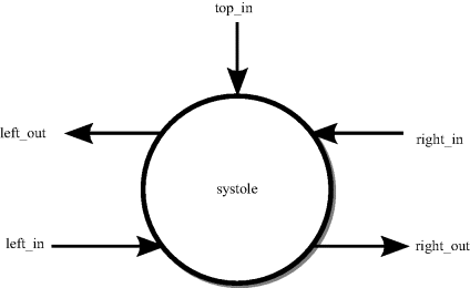
All the inputs are integers of the same precision and will be represented by type signed from numeric_std, with their size controlled by a generic parameter. In addition to the inputs and outputs shown in the figure, a clock input will be required.
The entity for this interface is:
library ieee;
use ieee.std_logic_1164.all;
use ieee.numeric_std.all;
entity systole is
generic (n : natural);
port (left_in, top_in, right_in : in signed(n-1 downto 0);
ck : in std_logic;
left_out, right_out : out signed(n-1 downto 0));
end;
The systole is a simple multiply-accumulate structure with a register to store the intermediate results. One of the inputs is fed through a register to the outputs directly. The internal architecture is shown in Figure 10.6.
Figure 10.6 Internal structure of the systole.

All the intermediate signals are the same precision as the inputs and outputs and so should also be parameterised by the generic parameter.
The architecture for the systolic processor is:
architecture behaviour of systole is
signal sum : signed(n-1 downto 0);
signal product : signed(2*n-1 downto 0);
begin
product <= left_in * top_in;
sum <= right_in + product(n-1 downto 0);
process
begin
wait until rising_edge(ck);
left_out <= sum;
right_out <= left_in;
end process;
end;
Note how a double length product is created as in intermediate signal, since the output of the multiply operator in numeric_std gives a double length result. This is then truncated to the required length by the slice in the addition, so that only the lower half of product is kept. The resize function was not used for the truncation because it was required that overflow causes wrap-around and the resize function for signed preserves the sign (see Section 6.4 for an explanation of the problems with the resize function).
The most significant bits of the product are not used in the circuit, so synthesis will remove them. Thus, all the datapaths in the solution are of equal width, specified by the generic parameter n.
Now that the systolic element has been designed, it is possible to complete the systolic multiplier.
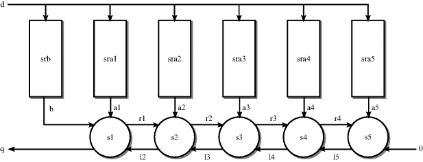
The multiplier is intended to multiply a 3 × 3 matrix by a 3-element vector. The systolic multiplier is illustrated by the block diagram in Figure 10.7. The data inputs are fed into the processor through a single 8-bit port, so part of the solution is to store the data and feed it to the array at the right time.
Figure 10.7 Data flow of the systolic multiplier.

In fact, the b elements are fed in 2 cycles before the a elements so that b(1) meets a(1,1) in the middle systole. The first result will emerge from the left-hand end of the array another 2 cycles later.
The first stage in the solution is to find a solution to the data input scheduling. This requires that the data samples are stored prior to being fed into the systolic array. the most appropriate solution here is to use shift registers with an enable control. When enabled, they act as first-in, last-out shifters. When disabled, they hold their values and output a zero to the systolic array.
The shifter circuit has the interface shown in Figure 10.8.
Figure 10.8 Interface to the shift register.
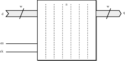
The shift register is parameterised in both word-width (w) and number of stages (n). The design of the shift register is:
library ieee;
use ieee.std_logic_1164.all, ieee.numeric_std.all;
entity shifter is
generic (w, n : natural);
port (d : in signed(w-1 downto 0);
ck, en : in std_logic;
q : out signed(w-1 downto 0));
end;
architecture behaviour of shifter is
type signed_array is array(0 to n) of signed(w-1 downto 0);
signal data : signed_array;
begin
data(0) <= d;
gen: for i in 0 to n-1 generate
process
begin
wait until ck'event and ck = '1';
if en = '1' then
data(i+1) <= data(i);
end if;
end process;
end generate;
q <= data(n) when en = '1' else (others => '0'),
end;
Note how the generate statement has been simplified by making the data array one element larger than necessary and using data(0) as the register input. This element is not registered since it is never used as the target of an assignment in a registered process. Only elements data(1) to data(n) will be registered.
The next stage is to create the basic structure of the systolic multiplier, at this stage without the controller that will synchronise the activities of the systoles and the shift registers. The structure of the systolic multiplier is shown in Figure 10.9.
Figure 10.9 Internal structure of the systolic multiplier.
For this example, all the datapaths will be 16-bit signed numbers.
The interface to the systolic multiplier is described by the following entity:
library ieee;
use ieee.std_logic_1164.all;
use ieee.numeric_std.all;
entity systolic_multiplier is
port (d : in signed (15 downto 0);
ck, rst : in std_logic;
q : out signed (15 downto 0));
end;
The architecture contains five component instances of the systole component and six instances of the shifter component, with different generic shift lengths reflecting the number of values to be stored in each shifter.
architecture behaviour of systolic_multiplier is
signal b, a1, a2, a3, a4, a5, r1, r2, r3, r4, l2, l3, l4, l5, nil
: signed (15 downto 0);
signal enb, ena1, ena2, ena3, ena4, ena5 : std_logic;
begin
nil <= (others => '0'),
s1 : entity work.systole
generic map (16) port map (b, a1, l2, ck, q, r1);
s2 : entity work.systole
generic map (16) port map (r1, a2, l3, ck, l2, r2);
s3 : entity work.systole
generic map (16) port map (r2, a3, l4, ck, l3, r3);
s4 : entity work.systole
generic map (16) port map (r3, a4, l5, ck, l4, r4);
s5 : entity work.systole
generic map (16) port map (r4, a5, nil,ck, l5, open);
srb : entity work.shifter
generic map (16, 3) port map (d, ck, enb, b);
sra1 : entity work.shifter
generic map (16, 1) port map (d, ck, ena1, a1);
sra2 : entity work.shifter
generic map (16, 2) port map (d, ck, ena2, a2);
sra3 : entity work.shifter
generic map (16, 3) port map (d, ck, ena3, a3);
sra4 : entity work.shifter
generic map (16, 2) port map (d, ck, ena4, a4);
sra5 : entity work.shifter
generic map (16, 1) port map (d, ck, ena5, a5);
end;
The final stage of the design is the design of the controller that synchronises the systolic multiplier. This will appear as processes in the structural description and controls the enable signals for the shift register components. The controller is basically a simple sequencer with decoding for the various enable signals. The synchronous reset input to the systolic multiplier will be used to simply reset the sequencer. There is no need for resets on any of the other components.
The controller is in two parts, a counter and a decoder. The counter is based on an enumeration type so that each control state can be given a meaningful name. The calculation proceeds in two phases: load the data into the shift registers; perform the calculation. It takes 12 clock cycles to load the shift registers and 9 clock cycles to perform the calculation, a total of 21 clock cycles. In principle, it should be possible to overlap the two phases, but for this example they will be kept separate for clarity. The results come out on the q output separated by zeros, with the first element of the result appearing on the fifth cycle of the calculation phase and the last on the ninth cycle.
In order to implement the counter, a new type and counter signal will need to be added to the architecture:
type state_type is
(ld_a11, ld_a12, ld_a13,
ld_a21, ld_a22, ld_a23,
ld_a31, ld_a32, ld_a33,
ld_b1, ld_b2, ld_b3,
calc1, calc2, calc3, calc4, calc5, calc6, calc7, calc8, calc9);
signal state : state_type;
The next stage is to design a counter for this type. It must have an external synchronous reset and must also reset to the start of the sequence after the last state. The counter is:
process
begin
wait until ck'event and ck = '1';
if rst = '1' or state = state_type'right then
state <= state_type'left;
else
state <= state_type'rightof(state);
end if;
end process;
The final part of the solution is the decoding logic, implemented as a combinational process containing a case statement that implements the decoding of the current state:
process (state)
begin
enb <= '0';
ena1 <= '0';
ena2 <= '0';
ena3 <= '0';
ena4 <= '0';
ena5 <= '0';
case state is
when ld_a11 => ena3 <= '1';
when ld_a12 => ena4 <= '1';
when ld_a13 => ena5 <= '1';
when ld_a21 => ena2 <= '1';
when ld_a22 => ena3 <= '1';
when ld_a23 => ena4 <= '1';
when ld_a31 => ena1 <= '1';
when ld_a32 => ena2 <= '1';
when ld_a33 => ena3 <= '1';
when ld_b1 => enb <= '1';
when ld_b2 => enb <= '1';
when ld_b3 => enb <= '1';
when calc1 => enb <= '1';
when calc2 => null;
when calc3 => enb <= '1'; ena3 <= '1';
when calc4 => ena2 <= '1'; ena4 <= '1';
when calc5 => enb <= '1'; ena1 <= '1';
ena3 <= '1'; ena5 <= '1';
when calc6 => ena2 <= '1'; ena4 <= '1';
when calc7 => ena3 <= '1';
when calc8 => null;
when calc9 => null;
end case;
end process;
Before the case statement, all the control signals are initially set to '0'. Within the case statement, these values are selectively overridden by a '1' for those control signals that are required to be set. This makes the case statement both simpler and clearer than setting all of the controls in all of the branches. Note the use of the null statements where there are no assignments in a branch of the case statement. For no particular reason, it is illegal in VHDL to have an empty branch, so the null statement overcomes this.
Horowitz, P. and Hill, W. (1989) The Art of Electronics, 2nd edn, Cambridge University Press, Cambridge, UK, ISBN 978-0-521370950.