5	Propagation of Light
	Natalia Dushkina

CONTENTS

5.1    Properties of Light

5.1.1    Maxwell’s Equations

5.1.2    Harmonic Waves and the Wave Equation

5.1.3    Nature of Light

5.1.3.1    Light Is a Three-Dimensional Plane Electromagnetic Wave

5.1.3.2    Light Is a Transverse Wave

5.1.3.3    Electric and Magnetic Vectors Are Perpendicular to Each Other

5.1.3.4    Light Polarization

5.1.3.5    Energy Flow and Poynting Vector

5.1.3.6    Irradiance

5.1.3.7    Photons, Radiation Pressure, and Momentum

5.1.3.8    Electromagnetic Spectrum

5.2    Propagation of Light in Isotropic Media

5.2.1    Propagation of Light in Dielectrics

5.2.2    Reflection and Refraction

5.2.2.1    Boundary Conditions

5.2.2.2    Laws of Reflection and Refraction

5.2.2.3    Fresnel Formulae

5.2.2.4    Normal Incidence

5.2.2.5    Degree of Polarization

5.2.2.6    Brewster Angle

5.2.2.7    Phase Relations

5.2.3  Total Internal Reflection of Light

5.2.3.1    Reflected Wave

5.2.3.2    Evanescent Wave

5.2.4    Dispersion

5.2.4.1    Dispersion in Dielectrics

5.2.4.2    Normal Dispersion

5.2.4.3    Anomalous Dispersion

5.2.4.4    Group Velocity of a Wave Packet

5.2.4.5    Color of Objects.

5.2.5  Propagation of Light in Metamaterials

References

This chapter presents a brief description of the fundamental properties of light as described by Maxwell’s electromagnetic (EM) theory and the laws governing the propagation of light in isotropic materials. The goal is to summarize some of the most often used concepts and expressions such as Maxwell’s equations, wave equation, energy flow, the Poynting vector, irradiance, reflection, refraction, and dispersion. We confine our discussion to isotropic and homogeneous materials, and mainly to nonconducting materials with linear properties. Comprehensive description of propagation of light in anisotropic media, as well as reflection and propagation of light in conducting media is given in Refs. [1,2]. This chapter concentrates on the wave character of light and does not consider the quantum nature of light. Coherence and polarization of light are not discussed in details here, because they are extensively described in Chapters 1 and 5, respectively. The detailed derivation of the final formulae and equations presented here can be found in Refs. [1,2,3,4,5]. For introduction to the EM theory of light one can refer, to Refs. [4,5,6,7,8,9,10], while more detailed description of the concepts of modern optics are given in Refs. [11,12,13,14,15]. The fundamentals of electrodynamics, which is the basis of Maxwell’s EM theory and some of the mathematical methods used are presented in Refs. [16,17,18,19]. The books of Shen [20] and Boyd [21] are possible introductory text to the principles of nonlinear optics and some introductory articles on metrological methods that employ nonlinear optics [20,21,22,23,24]. For the specifics of interaction of light with holographic media, as well as principles, techniques, and applications of optical holography, one could refer to the text of Hariharan [25]. For an introduction to biomedical optics and propagation of light in live tissues, one can start with the book of Splinter and Hooper [26]. References [27,28,29,30,31,32,33,34,35,36,37,38,39,40,41,42,43,44,45,46,47,48,49] are only a short list of the literature devoted to the principles of nano-optics, evanescent fields, near-field optical methods, and other optical methods for characterization of thin films or nano-structures. At the end of this chapter, the reader finds a brief introduction to the newly emerging and quickly developing field of artificially constructed metamaterials (MMs), which are of considerable interest because of their extraordinary EM properties [50,51,52,53,54,55,56,57,58,59,60,61,62,63,64,65,66,67,68,69,70,71,72,73,74]. There is a large amount of publications in all these areas and the ones referred to here are only a small fraction.

5.1    PROPERTIES OF LIGHT

5.1.1    MAXWELL’s EQUATIONS

Light is an EM wave. Its properties are described by a set of four equations, known as Maxwell’s equations [1,2,3]. Maxwell’s EM theory explains all optical phenomena except certain quantum phenomena, for instance, absorption and emission of light. Maxwell’s equations, given in a general form below, summarize the four basic laws of classical electrodynamics [16,17,18,18]:

$\text{div}D=\text{ρ}$

(5.1a)

$\text{div}B=0$

(5.1b)

$\text{curl }E=-\frac{\partial B}{\partial t}$

(5.1c)

$\text{curl }H=J+\frac{\partial D}{\partial t}$

(5.1d)

where

E and H are the electric and magnetic field vectors, respectively

ρ is the free charge density

J is the free current density

Vector fields D and B are the electric displacement and magnetic induction, respectively which describe the behavior of material media in the presence of external electric and magnetic fields.

Equation 5.1a represents Gauss’s law for electric field (free space): the outward electric flux integrated over a closed surface is proportional to the net electric charge enclosed by the surface. Equation 5.1b is Gauss’s law for magnetic field (free space): the outward magnetic flux integrated over a closed surface is zero. It implies the experimental fact that no isolated magnetic poles (magnetic monopoles) have ever been observed. Equation 5.1c is the mathematical representation of Faraday’s induction law for free space: a time-varying magnetic field induces an electric field. Equation 5.1d is Ampere’s law for free space, which states that a time-varying electric field induces a magnetic field. Equations 5.1a through d are valid for time-varying fields such as the electric and magnetic fields constituting an EM wave and relate the electric and magnetic fields with the sources (currents and charges) that produce them in matter. Maxwell’s equations do not account for fields that are constant in time and space and any such additional field should be added to the E and H fields. Since the electric field E and the magnetic induction B determine forces acting on a charge (or current), the actual physical observables are forces. The force exerted on a charge q moving with velocity v in an EM field (E, B) is given by the Lorentz force law:

$F=q\left(E+v\times B\right)$

(5.2)

The EM properties of the medium are described by the macroscopic polarization P and magnetization M, which are linked to the vectors E, D, H, and B according to

$D\left(r,t\right)={\text{ε}}_{0}E\left(r,t\right)+P\left(r,t\right)$

(5.3a)

$H\left(r,t\right)={\text{μ}}_0^{-1}B\left(r,t\right)-M\left(r,t\right)$

(5.3b)

These general equations are always valid because they do not impose conditions on the medium. The constants ε₀ and μ₀ are the electric permittivity and the permeability of free space, respectively, with values

${\text{ε}}_0=8.8542\times {10}^{-12}\frac{{\text{C}}^2}{\text{N}\cdot {\text{m}}^2}$

(5.4a)

and

${\text{μ}}_0=4\pi \times {10}^{-7}\frac{\text{N}\cdot {\text{s}}^2}{{\text{C}}^2}=1.2566\times {10}^{-6}\frac{\text{N}\cdot {\text{s}}^2}{{\text{C}}^2}$

(5.4b)

The behavior of matter under the influence of electric and magnetic fields is described by the material equations, which for a nondispersive, isotropic, and continuous medium have the form

$D=\text{ε}E$

(5.5a)

$B=\text{μ}H$

(5.5b)

$J_{\text{c}}=\text{σ}E$

(5.5c)

$P={\text{ε}}_0{\chi }_{\text{e}}E$

(5.5d)

$M={\chi }_{\text{m}}H$

(5.5e)

where

J_c denotes the induced conduction current density

χ_e and χ_m are the electric and magnetic susceptibility, respectively

Material parameters ε, μ, and σ are the permittivity, magnetic permeability, and specific conductivity, respectively

The permittivity ε and permeability μ describe the response of a homogeneous material to the electric and magnetic components, respectively, of a radiation of a given frequency. The permittivity and the magnetic permeability of the substance are expressed as ε = ε_rε₀ and μ=μ_rμ₀ respectively, where ε_r =ε/ε₀ and μ_r = μ/μ₀ are the values relative to vacuum. The relative permittivity of the material ε_r is also referred to as the dielectric constant. For nonmagnetic materials μ_r = 1. In this chapter, we consider only nonmagnetic materials, thus μ = μ₀.

An isotropic and homogeneous medium is one, whose properties at each point are independent of direction. Hence, the material parameters ε, μ, and σ of such a medium are constants. For anisotropic materials, their values in Equations 5.5 are replaced by tensors. Equations 5.5 describe a linear medium. In the case of nonlinear material, the right-hand sides contain terms of higher power. If the material parameters are functions of frequency, it said that the material exhibits temporal dispersion. In linear, isotropic, homogenous, and source-free media, the EM field is entirely defined by two scalar fields.

In a nonmagnetic, nonconducting material (J = 0, σ = 0) with no free charges (ρ = 0), the four Maxwell’s equations can be expressed only in terms of the E and B fields. In Cartesian coordinates, they become [1,2]

$\nabla \cdot E=0$

(5.6a)

$\nabla \cdot B=0$

(5.6b)

$\nabla \times E=-\frac{\partial B}{\partial t}$

(5.6c)

$\nabla \times B={\text{μ}}_0\text{ε}\frac{\partial E}{\partial t}$

(5.6d)

where the divergence and curl of a vector, for instance of the vector E, are

$\text{div}E=\nabla \cdot E=\frac{\partial E_x}{\partial x}+\frac{\partial E_y}{\partial y}+\text{}\frac{\partial E_z}{\partial z}$

(5.7a)

and

$\text{curl}E=\nabla \times E=\left(\frac{\partial E_z}{\partial y}-\frac{\partial E_y}{\partial z}\right)\widehat{x}+\left(\frac{\partial E_x}{\partial z}-\frac{\partial E_z}{\partial x}\right)\widehat{y}+\left(\frac{\partial E_y}{\partial x}-\frac{\partial E_x}{\partial y}\right)\widehat{z}$

(5.7b)

where $\widehat{x},\widehat{y}$, and $\widehat{z}$ are unit vectors in the x, y, and z directions.

5.1.2    HARMONIC WAVES AND THE WAVE EQUATION

Harmonic waves are produced by sources that oscillate in a periodic fashion and can be described by sine or cosine functions. A general harmonic wave in three-dimensions can be represented in a complex form as

$\text{ψ}\left(x,y,z,t\right)=A\left(x,y,z\right)e^{-i\left(\text{ω}t-k\cdot r+{\text{φ}}_0\right)},$

(5.8)

where A(x, y, z) is the amplitude of a wave with wavelength λ, frequency f, and a period T = 1/f. The wavelength and frequency determine the propagation constant k = 2π/λ and the angular frequency ω = 2πf of the wave. Since k is related to λ in the same way as the angular frequency ω=2π/T is related to the wave temporal period T, the wavelength λ can be considered as the spatial period of the wave, and the propagation constant k as the spatial frequency of the wave. In this context, the reciprocal of the wavelength 1/λ is called wave number. The argument of the exponent φ = ωt − k · r + φ₀ is the phase of the wave with φ₀ being the initial phase at t = 0 and r = 0. The phase φ depends on the spatial coordinates and time. Equation 5.8 describes a plane wave propagating in arbitrary direction determined by the propagation vector k, often also called wave vector. If the components of the propagation vector are (k_x, k_y, k_z), and (x, y, z) are the components of a point in space where the displacement ψ is considered, then the dot product is given by k · r =k_xx+k_yy+k_zz. The propagation vector k is normal to planes of constant phase defined by φ = const. and called wave fronts. If the phase φ is equal to integer multiples of 2π on these planes, a three-dimensional plane wave can be visualized as a train of wave fronts separated by one wavelength λ and moving with the wave speed v in direction given by k.

If the wave propagation is along the z direction, k · r becomes kz. During a time interval dt, the plane of constant phase moves a distance dz. The magnitude of the phase velocity v of the wave moving in z direction is

$\upsilon =\frac{dz}{dt}=\frac{\text{ω}}{k}=\lambda f$

(5.9)

The behavior of the phase difference Δφ at a given time between two points on the wave that are separated by a certain distance is important for evaluating the degree of coherence of the wave. If a monochromatic wave travels along the z direction with a wave vector k, then the phase difference between two points along z separated by distance Δz is Δφ = kΔz, ωt is the same at each point. If the phase difference Δφ = kΔz is equal to 0 or integer multiples of 2π, then these two points are in phase. A wave that maintains a constant phase difference in space and time exhibits high degree of coherence.

A wave described by Equation 5.8 satisfies the partial differential equation:

${\nabla }^2\Psi =\frac{1}{v^2}\frac{{\partial }^2\text{ψ}}{\partial t^2},$

(5.10)

which is the general form of the wave equation. Here v is the wave propagation velocity. The wave equation can be derived by employing the chain rule of partial differentiation to find the first and second spatial and temporal derivatives and equating the results for the two second derivatives. Plane waves have rectangular symmetry and are solutions of the wave equation (Equation 5.10), where the Laplacian operator is given in Cartesian coordinates by

${\nabla }^2=\frac{{\partial }^2}{\partial x^2}+\frac{{\partial }^2}{\partial y^2}+\frac{{\partial }^2}{\partial z^2}$

(5.11)

5.1.3    NATURE OF LIGHT

The four Maxwell’s equations for free space can be combined and manipulated to give as a final result the following two equations for the electric and magnetic vectors [1,4]:

${\nabla }^{2}E={\text{ε}}_0{\text{μ}}_0\frac{{\partial }^{2}E}{\partial t^2}$

(5.12a)

${\nabla }^{2}B={\text{ε}}_0{\text{μ}}_0\frac{{\partial }^{2}B}{\partial t^2}$

(5.12b)

These equations have the same form as the wave equation (Equation 5.10). In addition, the Laplacian operator acts on each component of E and B; hence, each component of the EM field obeys the scalar wave equation (Equation 5.10). This fact suggests the existence of harmonic EM waves that propagate in free space with velocity

$c=\frac{1}{\sqrt{{\text{ε}}_0{\text{μ}}_0}}=2.298\times {10}^8\text{m/s}$

(5.13)

The speed of light in vacuum is a fundamental constant with the exact value c = 299,792,458 m/s, which was defined by the Conference Générale des Poids et Mesures in 1983.

5.1.3.1    Light Is a Three-Dimensional Plane Electromagnetic Wave

This property follows from the fact that each component of E and B satisfies the differential wave equation (Equation 5.10). For EM waves (including light), ψ can be either of the varying electric or magnetic fields that constitute the wave. Thus, the variations of the electric and magnetic fields at point r on a plane perpendicular to the propagation vector k can be described with Equation 5.8 as

$E\left(r,t\right)=E_0\left(r\right){\text{e}}^{-i\left(\text{ω}t-k\cdot r+{\text{φ}}_0\right)}$

(5.14a)

and

$B\left(r,t\right)=B_0\left(r\right){\text{e}}^{-i\left(\text{ω}t-k\cdot r+{\text{φ}}_0\right)},$

(5.14b)

where E₀(r) and B₀(r) are the complex amplitudes of the electric and magnetic fields, respectively.

Equations 5.14a and b describe harmonic waves of the same frequency f (same ω) and propagate in arbitrary direction defined by the same propagation vector k; hence, have the same wavelength and speed in a given dielectric material

$v=\frac{1}{\sqrt{{\text{εμ}}_0}}$

(5.15)

5.1.3.2    Light Is a Transverse Wave

EM waves are transverse waves, because both vectors E and B lie in a plane that is perpendicular to the direction of propagation, determined by the direction of k. This follows from Maxwell’s equations (Equations 5.6a and b) when applied to the filed vectors E and B given by Equations 5.14a and b:

$\frac{\partial E_x}{\partial x}+\frac{\partial E_y}{\partial y}+\frac{\partial E_z}{\partial z}=i\left(k_x{E}_x+k_y{E}_y+k_z{E}_z\right)=ik\cdot E=0$

and

$\frac{\partial B_x}{\partial x}+\frac{\partial B_y}{\partial y}+\frac{\partial B_z}{\partial z}=i\left(k_x{B}_x+k_y{B}_y+k_z{B}_z\right)=ik\cdot B=0$

Since k · E = 0 and k · B = 0, both E and B must be perpendicular to k, which indicates that EM waves are transverse waves.

5.1.3.3    Electric and Magnetic Vectors Are Perpendicular to Each Other

This follows from the third Maxwell equation (Equation 5.6c). Assuming a wave traveling in positive z direction, with an electric vector E along the x-axis, we get from Equation 5.6c that $\widehat{y}\left(\partial E_x/\partial z\right)-\left(\partial B_y/\partial t\right)=i\text{ω}{B}_y$; thus, the only nonzero component of the magnetic field is along the y-axis. We can generalize this result using the cross product

$k\times E=\text{ω}B$

(5.16)

From Maxwell’s equations it follows that the harmonic variations of the electric and magnetic fields are always perpendicular to one another and to the direction of propagation given by k. In addition, in an isotropic nonconducting medium, the field magnitudes are related by

$E=\frac{\text{ω}}{k}B=vB$

(5.17)

or in free space, this equation becomes

$E=cB$

(5.18)

In vacuum and in air, the E and B fields oscillate in phase at any point in space and at any time. In a dissipative medium, however, a phase shift between the fields takes place. In good conductors, the magnetic field is much larger than the electric field and exhibits a phase delay of approximately 45°. In non-dissipative media, like glass for visible light, the E and B fields behave similar as in vacuum and are in phase.

5.1.3.4    Light Polarization

Since the two fields are interdependent, once one of them is specified, the direction and magnitude of the other can be obtained from the relations between them, that is, Equations 5.16 through 5.18. It is customary to specify the electric field and the direction of the electric field determines the polarization of the wave.

Let us consider again a wave traveling in positive z direction, with φ₀ = 0, and electric vector E along the x-axis, that is, the wave is polarized in the x direction. Such a wave can be represented by

$E=E_0\sin \left(kz-\text{ω}t\right)$

(5.19)

Using Equation 5.18, the magnetic field associated with this wave in free space is given by

$B=\frac{1}{c}{E}_0\sin \left(kz-\text{ω}t\right)$

(5.20)

According to Lorentz force law, Equation 5.2, the direction of the force exerted on a moving charge by the EM filed is defined by the direction of the electric vector E, thus, by the polarization of the wave. Since E and B lie in one plane which is perpendicular to k, we say that light is a plane polarized wave with polarization perpendicular to the direction of wave propagation. Equations 5.2 and 5.20 show that the electric force acting on the charge in general must be much larger than the magnetic force, which underlines the importance of the wave polarization in many optical phenomena and applications. The wave is said to be linearly polarized if the direction of the electric vector E remains constant in a given direction. The electric field vector, Equation 5.19, can be represented as the vector sum of two perpendicular waves E(z, t) = E_x(z, t) + E_y(z, t). For example, the light would be linearly polarized along the x direction, if the electric field oscillates always along the x direction. For a linear polarization, the amplitude and the direction of the electric field oscillation remain constant over time. If one component of the electric field, for instance this along the y direction, is always out of phase by π/2 with the x-component, but the amplitudes of both components are fixed, the polarization is said to be circular polarization. Both linear and circular polarizations are particular cases of the general case of elliptical polarization. The light is elliptically polarized when the electric field vector E(z, t) rotates and changes its magnitude over time. Natural light and light from sources other than lasers is randomly polarized, also called unpolarized light.

Since Chapter 5 is devoted entirely to polarization of light, we will neither discuss here the nature of the polarization of EM waves, nor will we describe here the ways of production of the different types of wave polarization.

5.1.3.5    Energy Flow and Poynting Vector

EM waves carry energy as they travel. An expression for the wave energy can be derived by using the analogy with a capacitor storing energy as an electric field and an inductor (a solenoid) storing energy as a magnetic field. By this analogy, the energy densities u_E and u_B (J/m³), associated with the static electric field of an ideal capacitor and the static magnetic field of an ideal solenoid are

$u_E=\frac{1}{2}{\text{ε}}_0{E}^2\text{and}{u}_B=\frac{1}{2}\frac{B^2}{{\text{μ}}_0}\left(\text{in free space}\right)$

(5.21)

for an EM wave, u_E = u_B. This result can be easily obtained from Equation 5.21 by replacing B with E/c from Equation 5.18:

$u_B=\frac{1}{2}\frac{B^2}{{\text{μ}}_0}=\frac{1}{2}\frac{1}{{\text{μ}}_0}{\left(\frac{E}{c}\right)}^2=\frac{1}{2}\frac{{\text{ε}}_0{\text{μ}}_0}{{\text{μ}}_0}{E}^2=\frac{1}{2}{\text{ε}}_0{E}^2=u_E$

(5.22)

The total energy density of the wave is the sum of the energy densities of its constituent electric and magnetic fields

$u=u_E+u_B=2u_E=2u_B$

(5.23)

which is equivalent to

$u={\text{ε}}_0{E}^2=\frac{B^2}{{\text{μ}}_0}={\text{ε}}_{0}cEB\text{θ}$

(5.24)

These two equations define the energy density of the EM field, that is, the energy per unit volume of the space where the EM field exists. A traveling wave carries energy and the rate at which energy is transported by the EM field defines the power of the EM wave.

The total energy transferred by the wave in a time Δt through an area A perpendicular to the direction of wave propagation is uΔV Here, ΔV is the volume determined by the cross section A and the length cΔt, that is, the distance traveled by the wave in a time Δt. Thus, the power of the wave can be expressed by

$\text{Power = }\frac{\text{Energy}}{\Delta t}=\frac{u\Delta V}{\Delta t}=\frac{u\left(c\Delta tA\right)}{\Delta t}=ucA$

(5.25)

The power per unit area (W/m²), or the energy flow per unit area per unit time, defines the energy flux S:

$S=\frac{ucA}{A}=uc$

(5.26)

By using Equation 5.24, the energy flux can also be expressed as

$S=\left({\text{ε}}_0{E}^2\right)c=\frac{1}{{\text{μ}}_0}EB={\text{ε}}_0{c}^{2}EB$

(5.27)

As the energy flow is in the direction of wave propagation, the energy flux S can be considered as a vector with magnitude given by Equation 5.27 and direction—the direction of wave propagation. Using the fact that E × B points in the direction of energy flow, the vector S can be expressed by the vectors of the electric and magnetic fields as

$S={\text{ε}}_0{c}^{2}E\times B=\frac{1}{{\text{μ}}_0}E\times B$

(5.28)

The vector S is called the Poynting vector.

5.1.3.6    Irradiance

In Chapter 1, we defined the irradiance as the radiant flux incident onto a unit area perpendicular to the direction of propagation of radiant energy. Irradiance is a measurable quantity and involves a measurement over some time interval, which is much larger than the period of variation of the EM field of optical frequencies (in the order of 10¹⁴ Hz for the visible spectrum). Since the electric and magnetic fields, therefore the magnitude of the Poynting vector, are rapidly varying functions of time, the measurement of the energy flux S inevitably involves time averaging. Hence, the irradiance is the time average of the magnitude of the Poynting vector:

$I=\langle \left|S\right|\rangle ={\text{ε}}_0{c}^2\langle E_0{B}_0{\sin }^2\left(k\cdot r-\text{ω}t\right)\rangle =\frac{1}{2}{\text{ε}}_0{c}^2{E}_0{B}_0\left[{\text{W/m}}^2\right]$

(5.29)

An alternative representation of irradiance is based on the alternative forms of energy density for free space, Equation 5.24:

$I=\frac{1}{2}{\text{ε}}_{0}c{E}_0^2=\frac{1}{2}\frac{c}{{\text{μ}}_0}{B}_0^2\left(\text{free space}\right)$

(5.30)

which within linear homogeneous isotropic material becomes

$I=\frac{1}{2}\text{ε}v{E}_0^2$

(5.31)

Usually, irradiance is denoted by E, as it was in Chapter 1. However, to avoid confusion of electric field with irradiance, we use here the symbol I for irradiance. Equation 5.29 has to employ the real representation of harmonic waves by sine and cosine functions, because the definition of Poynting vector, Equation 5.28, involves the product of two harmonic fields (E × B) and does not hold if they are given in complex form.

In summary, light is a three-dimensional plane polarized transverse EM wave, which carries energy and exerts a force on charges in the wave path; the magnitudes of the electric and magnetic fields are related by Equation 5.17 or 5.18, and the vectors E and B are oriented so that (E × B) points in the direction of energy flow.

5.1.3.7    Photons, Radiation Pressure, and Momentum

Maxwell’s EM theory cannot explain the processes of absorption and emission of light. These are quantum phenomena, which involve electronic transitions to and from quantized energy states, which lead to quantization of the absorbed and emitted radiations also. This reveals the quantum nature of light. In some optical phenomena, light behaves as a harmonic EM wave, while in others, it has to be considered a stream of energy quanta called photons. The phenomena absorption and emission of light are described in more details in Chapter 1, where it is shown that the energy of the absorbed or emitted photon is determined by the difference between the energies E_i and E_j of the energy levels involved in the electron transition. The photon energy cannot be subdivided and is given by

$E_{\text{ph}}=hf=h\frac{c}{\lambda }$

(5.32)

where

h is Planck’s constant (h = 6.626 × 10⁻³⁴ J · s = 4.136 × 10⁻¹⁵ eV · s)

f is the frequency

λ is the wavelength of the radiation

Specifically in semiconductor optics, the energy is expressed in electron volt rather than in joules. Hence, it is convenient to apply the following relation to find the energy into electron volt corresponding to a given wavelength in nanometer (10⁻⁹ m),

$E_{\text{ph}}\left[\text{eV}\right]=\frac{1240}{\lambda \left[\text{nm}\right]}$

(5.33)

Although photons have zero mass, they have nonzero momentum, which is determined by the photon energy

$p=\frac{E}{c}=\frac{h}{\lambda }=\hslash k$

(5.34)

where ħ = h/2π. The vector form of Equation 5.34, p = ħk, with k being the propagation vector reflects the fact that photon momentum is in the direction of energy flow.

When EM radiation impinges on an object’s surface, it interacts with the matter and exerts a force on the constituent charges. Since the force exerted on unit area defines pressure, the interaction of radiation with the surface results in radiation pressure [13]. Maxwell showed that the radiation pressure is determined by the energy density of the EM wave; thus, it can be expressed in terms of the magnitude of the Poynting vector. The average radiation pressure, which is the time average of the magnitude of the Poynting vector divided by the speed of light in vacuum, can be expressed with the irradiance of the impinging beam by

$\langle P\left(t\right)\rangle =\frac{\langle S\left(t\right)\rangle }{c}=\frac{I}{c}\left[\frac{\text{N}}{{\text{m}}^2}\right]$

(5.35)

On the other hand, force is the time rate of change of momentum, F = Δp/Δt; hence, radiation pressure is also related to the change of EM momentum of the wave reflected from or absorbed by the surface 〈P〉 =Δp/AΔt, where Δp is the amount of momentum transferred to the surface area A during the time interval Δt. The momentum transferred to the object per photon Δp is twice the photon momentum for total reflection from the surface and equal to the photon momentum for complete absorption. Since a beam of light with irradiance I has a photon flux per unit area equal to I/hv, the pressure exerted on the surface when the light is perfectly reflected from it can be expressed by

$\langle P\left(t\right)\rangle =\frac{I}{hv}\left[\frac{2h}{\lambda }\right]=\frac{2I}{c}$

(5.36)

Similarly, the pressure for complete absorption is given by 〈P(t)〉 =I/c, which is the same as Equation 5.35.

5.1.3.8    Electromagnetic Spectrum

The EM waves cover an extremely broad spectrum of wavelengths. We can detect only a very small segment of this spectrum directly through our sense of sight from approximately 750–400 nm.

EM waves are produced by oscillating charge distributions; thus, the frequency of the EM wave is determined by the frequency of the source of the wave. Equation 5.9 links the wave frequency and wavelength with the speed of propagation of the wave through a given medium (in vacuum, v = c). On the basis of the energy distribution among the EM waves of different frequencies, the spectrum is divided into six conceptual categories, as described below:

1.  Radio waves are low-frequencies (up to 10¹⁰ Hz), low-energy (up to 10⁻³ eV), long-wavelength (from kilometers for long radio waves to millimeters for microwaves) EM waves. This range includes AM and FM radio waves, broadcast television, and microwaves. Sometimes, microwaves, which extend from about 10⁹ up to about 3 × 10¹¹ Hz, and corresponding wavelengths of about 1 mm to 30 cm, are presented as a separate category. The signals are detected directly with antennas.

2.  Infrared (IR) radiation includes frequencies roughly from 3 × 10¹¹ to about 4 × 10¹⁴ Hz corresponding to wavelengths from 1 mm to about 750 nm. Photon energies range from 10⁻³ to about 1 eV. IR radiation is produced via thermal agitation of the molecules and any object at a temperature above the absolute zero will emit IR radiation. For example, a blackbody at room temperature emits radiation with wavelength maximum at around 10 μm.

3.  Visible range is the part of the EM spectrum that is detectable by the human eye. The term “light” refers to the visible EM radiation. The International Commission on Illumination has specified its limits to the frequency range from about 3.61 × 10¹⁴ to roughly 8.33 × 10¹⁴ Hz (which is the wavelength range from about 830 to 360 nm). Many texts, though, give narrower boundaries for the visible range, roughly from about 400 (violet) to 750 nm (red), corresponding to the visual response of the human eye. The emission of light results from rearrangement of the outer electrons in atoms and molecules. Photon energies are about 1–3 eV, which is sufficiently large to allow single-photon detection.

4.  Ultraviolet (UV) range covers frequencies approximately from 8 × 10¹⁴ to about 3.4 × 10¹⁶ Hz, with wavelengths from 380 down to 10 nm. The photon energies range from roughly 3.2 to 100 eV. These energy levels are large enough to ionize atoms in the upper atmosphere, to initiate photochemical reactions or to cause possible damage to living tissues. UV radiation results from electron transitions from highly excited states.

5.  X-rays are EM waves with wavelengths from 10 to about 10⁻⁴ nm (which is less than the atomic size) and frequencies from roughly 2.4 × 10¹⁶ to about 5 × 10¹⁹ Hz, and photon energies from about 100 eV up to 0.2 MeV. X-rays are produced from inner-shell atomic transitions when a metal target is bombarded with high-energy electrons.

6.  γ-Rays originate from nuclear transitions and have the shortest wavelengths (from 0.1 to 10⁻⁶ nm) and the highest energies (10⁴ to about 10¹⁹ eV). Because of these high energies, detection of single photons is possible. In addition, exposure of living tissues to x-rays and γ-rays can be extremely damaging.

5.2    PROPAGATION OF LIGHT IN ISOTROPIC MEDIA

5.2.1    PROPAGATION OF LIGHT IN DIELECTRICS

We consider here only a homogeneous isotropic dielectric media, the permittivity of which is independent of the coordinates as well as of time. For such a medium, Maxwell equations and all results derived for EM waves in vacuum are valid when ε₀ is replaced by ε. The wave velocity in a dielectric is

$v=\frac{1}{\sqrt{{\text{ε}}_{\text{r}}{\text{ε}}_0{\text{μ}}_0}}=\frac{c}{\sqrt{{\text{ε}}_{\text{r}}}}=\frac{c}{n}$

(5.37)

where

$n=\sqrt{{\text{ε}}_{\text{r}}}=\frac{c}{v}$

(5.38)

is the index of refraction and ε_r = ε/ε₀ is the relative permittivity. For magnetic materials, $n=\sqrt{{\text{ε}}_{\text{r}},{\text{μ}}_{\text{r}}}$, the wavelength in the dielectric is λ=λ_o/n and the wave number is k = 2π/λ. The energy density is given by

$u=\text{ε}{E}^2$

(5.39)

while the energy flux for a dielectric is

$S=uv=v\text{ε}{E}^2$

(5.40)

The irradiance of light within a homogeneous linear isotropic material is given by Equation 5.31.

5.2.2    REFLECTION AND REFRACTION

5.2.2.1    Boundary Conditions

The behavior of light at the interface between two different media is determined by the boundary conditions for the field vectors of the wave. In nonmagnetic materials with no free charges and conduction currents, these conditions require continuity of the tangential components of the electric and magnetic fields across the boundary [1]:

$\begin{array}{ccc}{E}_{2\text{τ}}=E_{1\text{τ}}& \text{and}& H_{2\text{τ}}=H_{1\text{τ}}\end{array}$

(5.41a)

followed automatically by the conditions for the normal components of D and B

$\begin{array}{ccc}{D}_{2n}=D_{1n}& \text{and}& B_{2n}=B_{1n}\end{array}$

(5.41b)

Here n and τ denote the normal and tangential component of the vectors, respectively. When the boundary conditions are imposed on the electric vectors of the incident, reflected, and refracted plane waves, the boundary conditions require that the strength of the electric field in the first medium, which consists of the field of the incident and reflected waves, is equal to the strength of the field in the second medium:

${\lfloor E_{0\text{i}}{\text{e}}^{-i\left({\text{ω}}_{i}t-k_{\text{i}}\cdot r\right)}+E_{0\text{r}}{\text{e}}^{-i\left({\text{ω}}_{r}t-k_{\text{r}}\cdot r\right)}\rfloor }_{\text{τ}}={\lfloor E_{0\text{t}}{\text{e}}^{-i\left({\text{ω}}_{\text{t}}t-k_{\text{t}}\cdot r\right)}\rfloor }_{\text{τ}}$

(5.42)

Here the subscripts i, r, and t denote the incident, reflected, and refracted (transmitted) waves. Equation 5.42 can be satisfied for arbitrary and independent variations of time and radius vector only if

${\text{ω}}_{\text{i}}t={\text{ω}}_{\text{r}}t={\text{ω}}_{\text{t}}t$

(5.43a)

$k_{\text{i}}\cdot r=k_{\text{r}}\cdot r=k_{\text{t}}\cdot r$

(5.43b)

Thus, ω_i = ω_r = ω_t, that is, the frequency of an EM wave, does not change as a result of reflection or refraction.

5.2.2.2    Laws of Reflection and Refraction

In geometrical optics, the direction of propagation of energy, which is in the direction of the wave propagation vector k, is depicted as a ray. The rays are always perpendicular to the wave fronts. Let us consider a ray impinging on the interface between two media with refractive indices n₁ and n₂, respectively. The origin of the radius vector r on the interface can be chosen in such a way that r is perpendicular to the vector k_i, that is, k_i · r = 0. Consequently, from Equation 5.43b, k_r · r = k_t · r = 0, which means that the vectors of the incident, reflected, and refracted rays, k_i, k_r, and k_t, all lie in the same plane. The plane specified by k_i and the normal to the boundary n is called plane of incidence. In Figure 5.1, the plane of incidence is the xz plane, the origin O of the rectangular Cartesian coordinate system is chosen at the point of incidence of the ray, and the direction of the z-axis is toward the second medium in which the refracted ray propagates. The vectors k_i, k_r, and k_t are applied at point O. The angles that the incident, reflected, and refracted rays make with Oz are θ_i, θ_r, and θ_t, respectively. The unit vector n is directed into the second medium along the normal to the interface. The tangential unit vector τ lies on the interface along the x-axis.

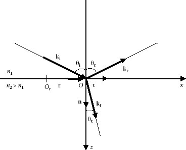
FIGURE 5.1  Incident, reflected, and refracted rays at a boundary between two dielectric media for external reflection (n₂ > n₁).

The laws of reflection and refraction follow from the boundary conditions. The law of reflection states that the wave vector k_r of the reflected wave lies in the plane of incidence and the angle of reflection is equal to the angle of incidence, or θ_r = −θ_i, when the angles are measured from the normal to the surface.

It follows from the boundary conditions that the ratio (sin θ_i/sin θ_t) is a constant and equal to the ratio of the wave velocities in both media as follows:

$\frac{\sin {\text{θ}}_{\text{i}}}{\sin {\text{θ}}_{\text{t}}}=\frac{v_1}{v_2}=\frac{n_2}{n_1}=n_{12}$

(5.44)

This equation can be rewritten as n₁ sin θ_i = n₂ sin θ_t and together with the statement that the refracted wave vector k_t is in the plane of incidence, constitute the Snell’s law of refraction. When a wave impinges on the interface between two media from the side of the optically rare medium, n₂ > n₁, the reflection is called external reflection. In this case, for every angle of incidence θ_i there is a real angle of refraction θ_t, which, by Equation 5.44 and sin θ_t < sin θ_i, is smaller than the incident angle θ_t < θ_i.

The refractive index is always greater than unity and depends not only on the substance but also on the wavelength of the light and temperature. For gases, it depends on the pressure also. Under normal conditions, the refractive index of gases differs from unity only by 10⁻³ or 10⁻⁴. For example, for air n = 1.0003, but if a very high accuracy is not required one can use for air n = 1 and the speed of light in vacuum. Equation 5.44 is valid when the magnetic properties of the media on different sides of the interface are identical μ₁ = μ₂. If this condition is not fulfilled and μ₁ ≠ μ₂, then Equation 5.44 becomes

$\frac{Z_1}{Z_2}=\frac{{\text{μ}}_1\sin {\text{θ}}_{\text{i}}}{{\text{μ}}_2\sin {\text{θ}}_{\text{t}}}$

(5.45)

where

$Z=\sqrt{\frac{\text{μ}}{\text{ε}}}$

(5.46)

is the wave impedance of the medium. For vacuum, $Z_0=\sqrt{{\text{μ}}_0/{\text{ε}}_0}=377\Omega$.

5.2.2.3    Fresnel Formulae

A plane wave linearly polarized in an arbitrary direction can be represented as a sum of two plane waves, one of which is polarized in the plane of incidence (denoted by subscript ║) and the other polarized in a plane perpendicular to the plane of incidence (denoted by subscript ⊥). The sum of the energy flux densities of these two waves should be equal to the energy flux density of the initial wave. Then, the incident, reflected, and refracted waves would be given by

$\begin{array}{cccc}{E}_{\text{i}}=E_{\text{i}║}+E_{\text{i}\perp },& E_{\text{r}}=E_{\text{r║}}+E_{\text{r}\perp },& \text{and}& E_{\text{t}}=E_{\text{t||}}\end{array}+E_{\text{t}\perp }$

(5.47)

According to the boundary conditions (Equations 5.41), the tangential components of the electric and magnetic fields should be continuous across the boundary. Hence, Equation 5.41a can be written for each polarization separately.

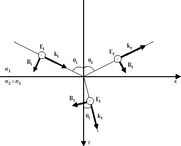
FIGURE 5.2  The incident wave is polarized perpendicularly to the plane of incidence.

Electric vector is perpendicular to the plane of incidence: This case is shown in Figure 5.2. It is seen that the tangential components of all electric field vectors are y-components, while for all magnetic field vectors they are x-components. The boundary condition for the electric vectors can be written as

$E_{0\text{i}}+E_{0\text{r}}=E_{0\text{t}}$

(5.48a)

and for the magnetic vectors

$-B_{0\text{i}}\cos {\text{θ}}_{\text{i}}+B_{0\text{r}}\cos {\text{θ}}_{\text{i}}=-B_{0\text{t}}\cos {\text{θ}}_{\text{t}}$

(5.48b)

Dividing both sides of Equation 5.48a by E_0i and using Equation 5.18 to substitute B in Equation 5.48b with (n/c)E, and then rearranging the terms, gives the Fresnel’s amplitude ratios for the reflected and transmitted waves:

${\left(\frac{E_{0\text{r}}}{E_{0\text{i}}}\right)}_{\perp }=\frac{n_1\cos {\text{θ}}_{\text{i}}-n_2\cos {\text{θ}}_{\text{t}}}{n_1\cos {\text{θ}}_{\text{i}}+n_2\cos {\text{θ}}_{\text{t}}}$

(5.49a)

${\left(\frac{E_{0\text{t}}}{E_{0\text{i}}}\right)}_{\perp }=\frac{2n_1\cos {\text{θ}}_{\text{i}}}{n_1\cos {\text{θ}}_{\text{i}}+n_2\cos {\text{θ}}_{\text{t}}}$

(5.49b)

When the law of refraction (Equation 5.44) is used, Equation 5.49 can also be written in the following alternative form, which does not contain the refractive indices:

${\left(\frac{E_{0\text{r}}}{E_{0\text{i}}}\right)}_{\perp }=-\frac{\sin \left({\text{θ}}_{\text{i}}-{\text{θ}}_{\text{t}}\right)}{\sin \left({\text{θ}}_{\text{i}}+{\text{θ}}_{\text{t}}\right)}$

(5.50)

${\left(\frac{E_{0\text{t}}}{E_{0\text{i}}}\right)}_{\perp }=\frac{2\sin {\text{θ}}_{\text{t}}\cos {\text{θ}}_{\text{i}}}{\sin \left({\text{θ}}_{\text{i}}+{\text{θ}}_{\text{t}}\right)}$

(5.51)

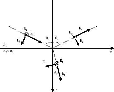
FIGURE 5.3  The incident wave is polarized parallel to the plane of incidence.

Electric vector is parallel to the plane of incidence: This case is shown in Figure 5.3. This time the tangential components of all magnetic field vectors are y-components, while the tangential components of all electric field vectors are x-components. The boundary condition for the electric vectors in this case is

$E_{0\text{i}}\cos {\text{θ}}_{\text{i}}+E_{0\text{r}}\cos {\text{θ}}_{\text{i}}=E_{0\text{t}}\cos {\text{θ}}_{\text{t}}$

(5.52a)

and for the magnetic vectors

$B_{0i}-B_{0r}=B_{0t}\text{which}\text{is also}{n}_1{E}_{0i}-n_1{E}_{0r}=n_2{E}_{0t}$

(5.52b)

Again, dividing both sides of Equation 5.52a and b by E_0i and rearranging, gives the Fresnel’s formulae for the amplitudes of the parallel polarization:

${\left(\frac{E_{0\text{r}}}{E_{0\text{i}}}\right)}_{\left|\right|}=\frac{n_2\cos {\text{θ}}_{\text{i}}-n_1\cos {\text{θ}}_{\text{t}}}{n_2\cos {\text{θ}}_{\text{i}}+n_1\cos {\text{θ}}_{\text{t}}}$

(5.53)

${\left(\frac{E_{0\text{t}}}{E_{0\text{i}}}\right)}_{\left|\right|}=\frac{2n_1\cos {\text{θ}}_{\text{i}}}{n_2\cos {\text{θ}}_{\text{i}}+n_1\cos {\text{θ}}_{\text{t}}}$

(5.54)

And the alternative forms are

${\left(\frac{E_{0\text{r}}}{E_{0\text{i}}}\right)}_{\left|\right|}=\frac{\tan \left({\text{θ}}_{\text{i}}-{\text{θ}}_{\text{t}}\right)}{\tan \left({\text{θ}}_{\text{i}}+{\text{θ}}_{\text{t}}\right)}$

(5.55)

${\left(\frac{E_{0\text{t}}}{E_{0\text{i}}}\right)}_{\left|\right|}=\frac{2\sin {\text{θ}}_{\text{t}}\text{cos}{\text{θ}}_{\text{i}}}{\sin \left({\text{θ}}_{\text{i}}+{\text{θ}}_{\text{t}}\right)\cos \left({\text{θ}}_{\text{i}}-{\text{θ}}_{\text{t}}\right)}$

(5.56)

If both media are transparent (no absorption), according to the principle of conservation of energy, the energies in the refracted and reflected waves should add up to the energy of the incident wave. The redistribution of the energy of the incident field between the two secondary fields is given by the reflection and transmission coefficients. The amount of energy in the primary wave, which is incident on a unit area of the interface per second, is given by

$J_i=I_i\cos {\text{θ}}_i=\frac{{\text{ε}}_{0}c}{2}{n}_1{\left|E_{0i}\right|}^2\cos {\text{θ}}_i,$

(5.57a)

And similarly, the energies of the reflected and refracted waves leaving a unit area of the interface per second are given by

$J_r=I_r\cos {\text{θ}}_i=\frac{{\text{ε}}_{0}c}{2}{n}_1{\left|E_{0r}\right|}^2\cos {\text{θ}}_i$

(5.57b)

$J_t=I_t\cos {\text{θ}}_t=\frac{{\text{ε}}_{0}c}{2}{n}_2{\left|E_{0t}\right|}^2\cos {\text{θ}}_t$

(5.57c)

where I_i, I_r, and I_t are the irradiances of the incident, reflected, and refracted waves, as defined by Equation 5.31. The ratios

$\mathcal{R}=\frac{J_{\text{r}}}{J_{\text{i}}}=\frac{{\left|E_{0\text{r}}\right|}^2}{{\left|E_{0\text{i}}\right|}^2}$

(5.58)

and

$\mathcal{T}=\frac{J_{\text{t}}}{J_{\text{i}}}=\frac{n_2}{n_1}\frac{\cos {\text{θ}}_{\text{t}}}{\cos {\text{θ}}_{\text{i}}}\frac{{\left|E_{0\text{r}}\right|}^2}{{\left|E_{0\text{i}}\right|}^2}$

(5.59)

are called reflectivity and transmissivity (or coefficients of reflection and transmission), respectively. It can be easily verified that for nonabsorbing media the energy flux density of the incident wave is equal to the sum of the energy flux densities of the reflected and transmitted waves. Hence, the law of conservation of energy is satisfied

$\mathcal{R}+\mathcal{T}=1$

(5.60)

The reflectivity and transmissivity depend on the polarization of the incident wave. If the vector E_i of the incident wave makes an angle α_i with the plane of incidence, then E_i║= E_i cos α_i and E_i⊥ = E_i sin α_i and Equations 5.58 and 5.59 can be rewritten using Equations 5.47 as

$\mathcal{R}=\frac{J_{\text{r}}}{J_{\text{i}}}=\frac{J_{\text{r|}}+J_{\text{r}\perp }}{J_{\text{i}}}={\mathcal{R}}_{\left|\right|}{\cos }^2{\text{α}}_{\text{i}}+{\mathcal{R}}_{\perp }{\sin }^2{\text{α}}_{\text{i}}$

(5.61)

and

$\mathcal{T}=\frac{J_{\text{t}}}{J_{\text{i}}}={\mathcal{T}}_{\left|\right|}{\cos }^2{\text{α}}_{\text{i}}+{\mathcal{T}}_{\perp }{\sin }^2{\text{α}}_{\text{i}},$

(5.62)

where

${\mathcal{R}}_{\left|\right|}=\frac{J_{\text{r||}}}{J_{\text{i|}}}=\frac{{\left|E_{0\text{r}}\right|}^2}{{\left|E_{0\text{i}}\right|}^2}=\frac{{\tan }^2\left({\text{θ}}_{\text{i}}-{\text{θ}}_{\text{t}}\right)}{{\tan }^2\left({\text{θ}}_{\text{i}}+{\text{θ}}_{\text{t}}\right)}$

(5.63a)

${\mathcal{R}}_{\perp }=\frac{J_{\text{r}\perp \text{|}}}{J_{\text{i}\perp }}=\frac{{\left|E_{0\text{r}\perp }\right|}^2}{{\left|E_{0\text{i}\perp }\right|}^2}=\frac{{\sin }^2\left({\text{θ}}_{\text{i}}-{\text{θ}}_{\text{t}}\right)}{{\sin }^2\left({\text{θ}}_{\text{i}}+{\text{θ}}_{\text{t}}\right)}$

(5.63b)

${\mathcal{T}}_{\left|\right|}=\frac{J_{\text{t|}}}{J_{\text{i|}}}=\frac{n_2}{n_1}\frac{\cos {\text{θ}}_{\text{t}}}{\cos {\text{θ}}_{\text{i}}}\frac{{\left|E_{0\text{t}\left|\right|}\right|}^2}{{\left|E_{0\text{i}\left|\right|}\right|}^2}=\frac{\sin 2{\text{θ}}_{\text{i}}\sin 2{\text{θ}}_{\text{t}}}{{\sin }^2\left({\text{θ}}_{\text{i}}+{\text{θ}}_{\text{t}}\right){\cos }^2\left({\text{θ}}_{\text{i}}-{\text{θ}}_{\text{t}}\right)}$

(5.64a)

${\mathcal{T}}_{\perp }=\frac{J_{\text{r}\perp }}{J_{\text{i}\perp }}=\frac{n_2}{n_1}\frac{\cos {\text{θ}}_{\text{t}}}{\cos {\text{θ}}_{\text{i}}}\frac{{\left|E_{0\text{t}\perp }\right|}^2}{{\left|E_{0\text{i}\perp }\right|}^2}=\frac{\sin 2{\text{θ}}_{\text{i}}\sin 2{\text{θ}}_{\text{t}}}{{\sin }^2\left({\text{θ}}_{\text{i}}+{\text{θ}}_{\text{t}}\right)}$

(5.64b)

Again we may verify that the reflection and transmission coefficients satisfy the law of energy conservation: R_║ + T_║ = 1 and R_⊥ + T_⊥ = 1. The dependence of the reflectivity and transmissivity on the angle of incidence θ_i, given by Equations 5.63 and 5.64 for external reflection, is shown in Figure 5.4.

When the magnetic properties of the media on the different sides of the interface are not identical, μ₁ ≠ μ₂, then n₁ and n₂ in Equations 5.63 and 5.64 should be replaced with Z₂ in Z₁ respectively as defined by Equation 5.46. As a result, the reflectivity and transmissivity become

$\begin{array}{l}{\mathcal{R}}_{\left|\right|}={\left(\frac{Z_1\cos {\text{θ}}_{\text{i}}-Z_2\cos {\text{θ}}_{\text{t}}}{Z_1\cos {\text{θ}}_{\text{i}}+Z_2\cos {\text{θ}}_{\text{t}}}\right)}^2\hfill \\ {\mathcal{R}}_{\perp }={\left(\frac{Z_2\cos {\text{θ}}_{\text{i}}-Z_1\cos {\text{θ}}_{\text{t}}}{Z_2\cos {\text{θ}}_{\text{i}}+Z_1\cos {\text{θ}}_{\text{t}}}\right)}^2\hfill \end{array}$

(5.65)

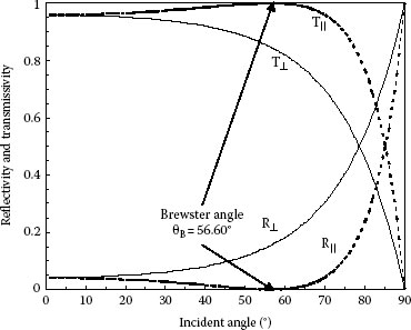
FIGURE 5.4  Fresnel’s reflection and transmission from glass in air, n₁ < n₂: n₁ = 1.0003 (glass BK 7) and n₂ = 1.5167 (for the sodium D line λ = 589.3 nm). Brewster angle θ_B = 56.60°.

$\begin{array}{l}{\mathcal{T}}_{\left|\right|}=\frac{4Z_1{Z}_2\cos {\text{θ}}_{\text{i}}\cos {\text{θ}}_{\text{t}}}{{\left(Z_1\cos {\text{θ}}_{\text{i}}+Z_2\cos {\text{θ}}_{\text{t}}\right)}^2}\hfill \\ {\mathcal{T}}_{\perp }=\frac{4Z_1{Z}_2\cos {\text{θ}}_{\text{i}}\cos {\text{θ}}_{\text{t}}}{{\left(Z_2\cos {\text{θ}}_{\text{i}}+Z_1\cos {\text{θ}}_{\text{t}}\right)}^2}\hfill \end{array}$

(5.66)

5.2.2.4    Normal Incidence

In the case of normal incidence, θ_i = 0, consequently θ_t = 0, and the expressions for the reflectivity and transmissivity are identical for both polarization components:

$\mathcal{R}={\left(\frac{n_2-n_1}{n_2+n_1}\right)}^2$

(5.67)

$\mathcal{T}=\frac{4n_1{n}_2}{{\left(n_2+n_1\right)}^2}$

(5.68)

It is obvious that the smaller the difference in the optical densities of the two media, the less energy is carried away by the reflected wave.

For media with magnetic properties, the coefficients (Equations 5.67 and 5.68) for normal incidence become

$\mathcal{R}={\left(\frac{{\text{μ}}_1{n}_2-{\text{μ}}_2{n}_1}{{\text{μ}}_1{n}_2+{\text{μ}}_2{n}_1}\right)}^2$

(5.69)

$\mathcal{T}={\left(\frac{2{\text{μ}}_2{n}_1}{{\text{μ}}_1{n}_2+{\text{μ}}_2{n}_1}\right)}^2$

(5.70)

5.2.2.5    Degree of Polarization

The variation in the polarization of light upon reflection or refraction is described by the degree of polarization:

$P=\frac{I_{\perp }-I_{\left|\right|}}{I_{\perp }+I_{\left|\right|}}$

(5.71)

where I_⊥ and I_║ are the irradiances of the perpendicular and parallel polarization components constituting the reflected or refracted beam, respectively. For unpolarized light, P = 0. For completely polarized light, P = 1, if the vector E is perpendicular to the plane of incidence and P = −1, if the vector E lies in the plane of incidence.

5.2.2.6    Brewster Angle

There is a special angle of incidence for which the sum of the incident angle and the refracted angle is 90°. When θ_i + θ_t = π/2, the denominator in Equation 5.55 turns to infinity, since tan (θ_i + θ_t) → ∞, and consequently R_║ = 0, while Equation 5.56 gives T_║ = 1. This angle of incidence θ_i = θ_B is called Brewster angle. Since the angle of reflection is equal to the angle of incidence, we can write θ_r + θ_t = π/2; from where it follows that when light strikes a surface at the angle of Brewster, the reflected and transmitted rays are also perpendicular to each other. Using this relation and the law of refraction gives

$\tan {\text{θ}}_{\text{B}}=\frac{n_2}{n_1}$

(5.72)

The zero value of the curve for the parallel component in Figure 5.4 corresponds to the Brewster angle for glass θ_B = 56.60°. If light is incident at Brewster angle θ_B, the reflected wave contains only the electric field component perpendicular to the plane of incidence, since R_║ = 0. Thus, the reflected light is completely polarized in the plane of incidence. Figure 5.4 shows that if the electric vector of the incident wave lies in the plane of incidence, all the energy of the wave incident at Brewster angle will be transferred into the transmitted wave, since there is no reflected wave with parallel polarization. Reflection at the Brewster angle is one of the ways of obtaining linearly polarized light.

Brewster angle can be experimentally determined by measuring the intensity of the parallel component of the reflected light by varying the angle of incidence continuously around the Brewster angle. Measurements of zero type (monitoring the intensity) are more precise and convenient than precise monitoring of the angle of incidence. At θ_i = θ_B, the intensity of the reflected wave with parallel polarizations should turn to zero according to Fresnel’s formulae for reflection. However, in reality, the intensity of the parallel component of the reflected wave does not become zero. The reason for this is that Fresnel’s formulae are derived when reflection and refraction take place at a mathematical boundary between two media. Actually, reflection and refraction take place over a thin surface layer with thickness about the interatomic distances. The properties of the transition layer differ from the properties of the bulk material, and therefore, the phenomena of reflection and refraction do not result in an abrupt and instantaneous change of the parameters of the primary wave, as described by the Fresnel’s formulae. This is also a consequence of the fact that Maxwell’s equations are formulated under the assumption that the medium is continuous and cannot describe accurately the process of reflection and refraction in the transition layer. As a result, for an incident wave of only perpendicular polarization, the wave reflected at Brewster angle is found to be elliptically polarized, instead of only linear polarization (perpendicular polarization) as Fresnel’s formulae predict. The deviations from Fresnel’s formulae due to the transition layer for angles other than the Brewster angle are hard to observe.

5.2.2.7    Phase Relations

The alternative forms (Equations 5.50, 5.51, 5.55, and 5.56) are more convenient when analyzing the phase of the reflected and refracted waves in respect with the incident wave.

Refraction: Since E_t║ and E_t⊥ have the same signs as E_i║ and E_i⊥, there is no change in the phase of the refracted waves for both polarizations. This means that under all conditions the refracted wave has the same phase as the incident wave.

Reflection: Depending on the conditions of reflection, the reflected wave may exhibit a change in phase:

1.  External reflection (a wave is incident at an interface from the optically rarer medium, n₁ < n₂ and θ_t < θ_i)

a.  Perpendicular polarization: At any angle of incidence, the phase of the perpendicular component of the electric field in the reflected wave changes by π, that is, E_r⊥ and E_i⊥ have opposite phases at the interface. This follows from Equation 5.50, which shows that at θ_t < θ_i the signs of E_r⊥ and E_i⊥ are different and the phases therefore differ by π. This means that the direction of the E_r⊥ is opposite to that shown in Figure 5.2.

b.  Parallel polarization: For electric vector oscillating in the plane of incidence, the phase change depends upon the angle of incidence. The ratio (E_0r/E_0i)_║ in Equation 5.55 is positive for θ_i < θ_B, and negative for θ_i > θ_B (θ_i + θ_t > π/2). This means that at Brewster angle the phase of the parallel component E_r║ abruptly changes to π. For incident angles smaller than the Brewster angle, θ_i < θ_B, the phase of the reflected wave (parallel polarization) is opposite to the phase of the incident wave, and does not change for θ_i > θ_B; thus, the reflected and incident waves have the same phases when θ_i > θ_B (i.e., at θ_i > θ_B the phase of the magnetic field changes by π).

2.  Internal reflection (a wave is incident at the interface from an optically denser medium, n₁ > n₂). The phase change is just the opposite of external reflection:

a.  Perpendicular polarization: At any angle of incidence, the phase of the perpendicular component of the electric field of the wave remains the same (i.e., in this case, the phase of the magnetic field changes by π).

b.  Parallel polarization: The phase of the parallel component remains unchanged for angles of incidence smaller than Brewster angle, θ_i < θ_B, and changes by π for angles of incidence exceeding θ_B (thus, the phase of the magnetic filed vector in the reflected wave does not change).

5.2.3    TOTAL INTERNAL REFLECTION OF LIGHT

When light impinges on the interface from the optically denser medium, n₁ > n₂, there is an angle of incidence, θ_i for which according to Equation 5.44 the refracted ray emerges tangent to the surface, θ_t = 90°. This angle is called critical angle θ_c. The critical angle is determined from Snell’s law by substituting θ_t = 90°:

$\sin {\text{θ}}_{\text{c}}=\frac{n_2}{n_1}=n_{12}\left(n_2<n_1\right)$

(5.73)

In this case, the angles of refraction θ_t have real values only for those incident angles θ_i, for which sin θ_i < n₁₂. When the angle of incidence is larger than the critical angle, total internal reflection takes place. For a glass/air interface with n_glass = 1.52, θ_c = 41.1°, the fact that θ_c is less than 45° makes it possible to use the hypotenuse of a triangular prism with angles 45°, 45°, and 90° as a totally reflecting surface.

5.2.3.1    Reflected Wave

For incidence angles smaller than the critical angle θ_i < θ_c, the Fresnel’s formulae (Equations 5.50, 5.55, and 5.63) are used, and the phase relations discussed for internal reflection above are valid. The case of total internal reflection, when the angle of incidence exceeds the critical angle, requires a special consideration.

Amplitude ratios: The law of refraction sin θ_t = sin θ_i/n does not give a real value for θ_t, when θ_i > θ_c. Therefore, cos θ_t in the Fresnel’s formulae is a complex quantity, represented as

$\cos {\text{θ}}_{\text{t}}=\pm \sqrt{{\sin }^2{\text{θ}}_{\text{t}}-1}=\pm i\sqrt{\frac{{\sin }^2{\text{θ}}_{\text{i}}}{n^2}-1}$

(5.74)

where for clarity and simplicity n₁₂. is replaced with n. The modified Fresnel’s amplitude ratios for internal reflection when θ₁ > θ_c have the form:

$\begin{array}{ll}{\left(\frac{E_{0\text{r}}}{E_{0\text{i}}}\right)}_{\left|\right|}\hfill & =\frac{n^2\cos {\text{θ}}_{\text{i}}-i\sqrt{{\sin }^2{\text{θ}}_{\text{i}}-n^2}}{n^2\cos {\text{θ}}_{\text{i}}+i\sqrt{{\sin }^2{\text{θ}}_{\text{i}}-n^2}}\hfill \\ {\left(\frac{E_{0\text{r}}}{E_{0\text{i}}}\right)}_{\perp }\hfill & =\frac{\cos {\text{θ}}_{\text{i}}-i\sqrt{{\sin }^2{\text{θ}}_{\text{i}}-n^2}}{\cos {\text{θ}}_{\text{i}}+i\sqrt{{\sin }^2{\text{θ}}_{\text{i}}-n^2}}\hfill \end{array}$

(5.75)

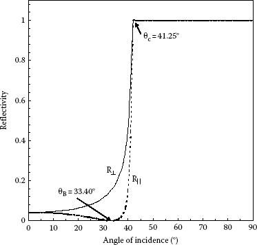
FIGURE 5.5  Internal reflection from glass/air interface: n₁ = 1.5167 (for the sodium D line λ = 589.3 nm, glass BK 7) and n₂ = 1.0003.

The reflectivity, which gives the ratio of the intensities of the reflected and incident waves, in this case would be the product of the amplitude ratio (Equation 5.75) and its complex conjugate, which leads to R_║ = R_⊥ = 1. Hence, the irradiance of the reflected light is equal to the irradiance of the incident light, independent of polarization; therefore, it is said that the wave is totally reflected in the first medium. The reflectivity for internal incidence is shown in Figure 5.5.

Phase relations: When the incident angle exceeds the critical angle θ_i > θ_c, we can say that the amplitudes of the reflected and incident waves are equal,

$\begin{array}{l}\begin{array}{ccc}{\left|\frac{E_{0\text{r}}}{E_{0\text{i}}}\right|}_{\left|\right|}=1& \text{or}& \left|E_{0\text{r|}}\right|=\left|E_{0\text{i|}}\right|\end{array}\hfill \\ \begin{array}{ccc}{\left|\frac{E_{0\text{r}}}{E_{0\text{i}}}\right|}_{\perp }=1& \text{or}& \left|E_{0\text{r}\perp }\right|=\left|E_{0\text{i}\perp }\right|\end{array}\hfill \end{array}$

(5.76)

and set

$\begin{array}{ccc}\frac{E_{\text{r||}}}{E_{\text{i|}}}={\text{e}}^{i{\text{δ}}_{\left|\right|}}& \text{and}& \frac{E_{\text{r}\perp }}{E_{\text{i}\perp }}\end{array}={\text{e}}^{i{\text{δ}}_{\perp }}$

(5.77)

The formulae for the phase relation between the reflected and incident waves would be

$\begin{array}{l}\tan \frac{{\text{δ}}_{\left|\right|}}{2}=-\frac{\sqrt{{\sin }^2{\text{θ}}_{\text{i}}-n^2}}{n^2\cos {\text{θ}}_{\text{i}}}\hfill \\ \tan \frac{{\text{δ}}_{\perp }}{2}=-\frac{\sqrt{{\sin }^2{\text{θ}}_{\text{i}}-n^2}}{\cos {\text{θ}}_{\text{i}}}\hfill \end{array}$

(5.78)

The relative phase difference between both polarization states δ = δ_⊥ − δ_║ is then given by

$\tan \frac{\text{δ}}{2}=\frac{\cos {\text{θ}}_{\text{i}}\sqrt{{\sin }^2{\text{θ}}_{\text{i}}-n^2}}{{\sin }^2{\text{θ}}_{\text{i}}}$

(5.79)

Maximum value of the relative phase difference can be found by differentiating Equation 5.79 with respect to the incident angle θ_i and setting it zero, $\frac{\text{d}}{{\text{dθ}}_{\text{i}}}\left(\tan \frac{\text{δ}}{2}\right)=0$. This leads to a relation between θ_i and the relative refractive index, that has to be satisfied in order to get the maximum value of the relative phase difference:

${\sin }^2{\text{θ}}_{\text{i}}=\frac{2n^2}{1+n^2}$

(5.80)

And the maximum value of the relative phase difference is

$\tan \frac{{\text{δ}}_{\max }}{2}=\frac{1-n^2}{2n}$

(5.81)

The case δ = δ_⊥ − δ_║ = 90° is of particular interest for practical applications. It allows producing circularly polarized light from linearly polarized light that undergoes total internal reflection. For this purpose, the incident light should be linearly polarized at an angle of 45° with respect to the incidence plane. This guarantees equal amplitudes of the electric field for both polarization components of the incident wave, |E_0i║| = |E_0i⊥|, and by Equation 5.76 equal amplitudes of both polarizations in the reflected wave, |E_r║| = |E_r⊥|. In order to obtain relative phase difference of π/2 (δ = δ_⊥ − δ_║ = 90°) with a single reflection from the boundary, the relative refractive index should be less than 0.414 (from tan(π/4) = 1<(1−n²)/2n, i.e., $n_{12}<\sqrt{2}-1=0.414$). If one of the media is air, then the other should have a refractiveindex of at least 2.42. Although there are some transparent materials with such a large refractive index, it is cheaper and more practical to use two total reflections on glass. Fresnel used a glass rhomb with an angle α = 54°37′, which provided an angle of incidence θ_i also equal to 54°37′ and two total reflections to demonstrate this method.

For materials with magnetic properties, the amplitude and phase relations for total internal reflection become

$\begin{array}{ll}{\left(\frac{E_{\text{r}}}{E_{\text{i}}}\right)}_{\left|\right|}\hfill & =\frac{Z_1\cos {\text{θ}}_{\text{i}}-i{Z}_2\left(s/k_2\right)}{Z_1\cos {\text{θ}}_{\text{i}}+i{Z}_2\left(s/k_2\right)}\hfill \\ {\left(\frac{E_{\text{r}}}{E_{\text{i}}}\right)}_{\perp }\hfill & =\frac{Z_2\cos {\text{θ}}_{\text{i}}-i{Z}_1\left(s/k_2\right)}{Z_2\cos {\text{θ}}_{\text{i}}+i{Z}_1\left(s/k_2\right)}\hfill \end{array}$

(5.82)

$\begin{array}{l}\tan \frac{{\text{δ}}_{\left|\right|}}{2}=-\frac{Z_2\left(s/k_2\right)}{Z_1\cos {\text{θ}}_{\text{i}}}\hfill \\ \tan \frac{{\text{δ}}_{\perp }}{2}=-\frac{Z_1\left(s/k_2\right)}{Z_2\cos {\text{θ}}_{\text{i}}}.\hfill \end{array}$

(5.83)

where s is explained in the next section.

5.2.3.2    Evanescent Wave

The modified Fresnel’s ratios suggest that the energy of the incident wave is totally reflected back to the first medium. However, the EM field of the incident wave penetrates into the second medium and generates a wave that propagates along the interface of the two media. The energy carried by this wave flows to and fro, and although there is a component of the Poynting vector in the direction normal to the boundary, its time average vanishes. This implies that there is no lasting flow of energy into the second medium.

Let us consider the x-axis along the interface between the two media, and z-axis along the normal to the interface. Let the wave that penetrates into the optically less dense medium propagate along the positive direction of the x-axis. Such a wave can be described by [28]:

$E_{\text{t}}=E_{0\text{t}}\exp \left(-sz\right)\exp \left[-i\left(\text{ω}t-k_{1}x\sin {\text{θ}}_{\text{i}}\right)\right]$

(5.84)

where

$s=k_2{\left[{\left(\frac{n_1}{n_2}\right)}^2{\sin }^2{\text{θ}}_{\text{i}}-1\right]}^{1/2}=\frac{n_2\text{ω}}{c}{\left[{\left(\frac{\sin {\text{θ}}_{\text{i}}}{\sin {\text{θ}}_{\text{c}}}\right)}^2-1\right]}^{1/2}$

(5.85)

The amplitude E_0t exp(−sz) of the wave decreases exponentially upon moving from the interface into the second medium. Therefore, this wave is called evanescent wave. The distance at which the amplitude of the wave decreases by a factor of e is called penetration depth, d_p:

$d_{\text{p}}=s^{-1}=\frac{{\lambda }_2}{2\pi }{\left[{\left(\frac{n_1}{n_2}\right)}^2{\sin }^2{\text{θ}}_{\text{i}}-1\right]}^{-1/2}$

(5.86)

The effective depth of penetration is on the order of a wavelength (d_p ~ λ₂/2π). The evanescent wave has very special properties. It is not a plane wave because its amplitude is not constant in a plane perpendicular to the direction of its propagation. This wave is not transversal wave either since the component of the electric vector in the direction of propagation does not vanish [1]. The phase velocity of the penetrating disturbance

$v_{2x}=\frac{\text{ω}}{k_1\sin {\text{θ}}_{\text{i}}}=\frac{\sin {\text{θ}}_{\text{c}}}{\sin {\text{θ}}_{\text{i}}}{v}_2$

(5.87)

is also not constant. The phase velocity v_2x is smaller than the velocity of the wave in the second medium v₂. The radiation penetrating into the second medium can be demonstrated by using frustrated total reflection [29] produced by two prisms separated by a distance of about a quarter of a wavelength, as shown in Figure 5.6. This way, the energy of the evanescent wave can couple into the second prism before damping to zero. The width of the gap determines the amount of the transmitted energy, which can be measured for quantitative description of the effect. In addition, the ray returns to the first medium at a point, which is displaced parallel to the interface by a distance d relative to the point of incidence, as shown in Figure 5.7. This displacement is called Goos–Hänchen shift and is less than a wavelength [30]. The frustrated total reflection allows also measurement of the Goos–Hänchen shift. Quantitative comparison of the theory of frustrated total reflection with experiment for the optical wavelengths shows that the values d/λ range from 0.25 to 1 approximately, which corresponds to values from 80% to 0.008% for the transmission of the evanescent wave into the second prism [29]. The significance of the Goos–Hänchen shift becomes evident with the emergence of near-field microscopy and lithography. Another way to demonstrate the penetrating radiation is by observing directly the luminescence from a thin fluorescent layer deposited on the second prism in the same configuration.

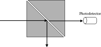
FIGURE 5.6  Frustrated total reflection.

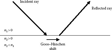
FIGURE 5.7  Positive Goos–Hänchen shift on total reflection. (After Lakhtakia, A., Int. J. Electron. Commun., 58, 229, 2004.)

In summary, in the case of total reflection, the energy flux of the incident wave is totally reflected and the components of the electric field parallel and perpendicular to the plane of incidence undergo different phase changes. The wave penetrates the second medium to a depth of about a wavelength, and propagates in the second medium along the interface with a phase velocity which is smaller than the velocity of the wave in the second medium. The totally reflected ray returns to the first medium at a point, which is displaced relative to the point of incidence.

5.2.4    DISPERSION

5.2.4.1    Dispersion in Dielectrics

The dielectric constant is ε_r; hence, the index of refraction and velocity of EM waves in a dielectric depend on frequency. This phenomenon is called dispersion. Since the various frequencies that constitute the wave propagate with different speeds, the effect of dispersion can be easily demonstrated with white light refracted by a prism resulting in a spread of colors. Figure 5.8 shows the variation of refractive index with wavelength within the visible range for different optical materials. The value of n typically decreases with increasing wavelength and thus increases with increasing frequency. Light of longer wavelength usually has greater speed in a material than light of shorter wavelength.

Dispersion is a consequence of the frequency dependence of atomic polarization of the material, which is determined by the dipole moments of the constituent atoms or molecules. A dipole is a pair of a negative −Q and a positive +Q charges with equal magnitudes and separated by a distance s. The dipole moment is a vector with magnitude Qs and direction pointing from −Q to +Q:

$p=Qs$

(5.88)

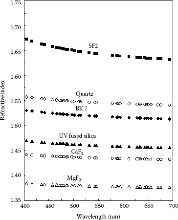
FIGURE 5.8  Variation of refractive index with wavelength. (Courtesy of Newport Corporation, Richmond, VA.)

An external electric field can induce dipole moments in dielectrics with symmetrical constituent molecules, or can align the permanently existing and randomly oriented dipole moments in dielectrics composed by asymmetrical molecules. An example for asymmetrical molecule with permanent dipole moment is the water molecule. The macroscopic polarization of a dielectric material is defined by the dipole moment per unit volume [1,2,3]:

$P=Np=N\frac{e^{2}E}{m\left({\text{ω}}_0^2-{\text{ω}}^2-i\gamma \text{ω}\right)}$

(5.89)

where

$p=e^{2}E/\left[m\left({\text{ω}}_0^2-{\text{ω}}^2-i\gamma \text{ω}\right)\right]$ is the dipole moment of an atom induced by the electric field of a harmonic wave with frequency ω

e and m are the charge and the mass of an electron, respectively

N (m⁻³) is the number of dipole moments per unit volume, which is the number of electrons per unit volume with natural frequency ω₀

γ describes the damping of oscillations

The macroscopic polarization P is a complex quantity with frequency-dependent and time-varying behavior. For linear dielectrics, it is proportional to the electric field E via the material Equation 5.5d, P = ε₀χ₁E. Combining this expression with Equation 5.89 gives the linear complex dielectric susceptibility as

${\chi }_1=\frac{e^{2}N}{{\text{ε}}_{0}m\left({\text{ω}}_0^2-{\text{ω}}^2-i\gamma \text{ω}\right)}$

(5.90)

Taking into account Equations 5.3a and 5.5a, the frequency-dependent permittivity can be written as

${\text{ε}}_{\text{ω}}={\text{ε}}_0+\frac{e^2}{{\text{ε}}_{0}m}\cdot \frac{N}{{\text{ω}}_0^2-{\text{ω}}^2-i\gamma \text{ω}}$

(5.91)

Consequently, the refractive index would be

${\widehat{n}}_{\text{ω}}^2={\text{ε}}_{\text{rω}}=1+\frac{e^2}{{\text{ε}}_{0}m}\cdot \frac{N}{{\text{ω}}_0^2-{\text{ω}}^0-i\text{γω}}$

(5.92)

where ε_rω =ε_ω/ε₀ is the frequency-dependent relative permittivity. Equation 5.92 shows that the index of refraction and hence the velocity of EM waves in a given material depend upon frequency. The refractive index is a complex quantity:

${\widehat{n}}_{\text{ω}}=n_{\text{ω}}+i{\text{ξ}}_{\text{ω}}$

(5.93)

where n_ω and ξ_ω are the real and imaginary part of ${\widehat{n}}_{\text{ω}}$ as both depend upon frequency ω = 2πf If in addition to the electrons with natural oscillation frequency ω₀, there are also electrons with other natural oscillation frequency ω_0i, they also contribute to the dispersion and have to be taken into account. If N_i is the number density of the electrons with natural oscillation frequency ω_0i, the refractive index can be written as the sum:

$n_{\text{ω}}^2=1+\frac{e^2}{{\text{ε}}_{0}m}{\displaystyle \sum _i\frac{N_i}{{\text{ω}}_{0\text{i}}^2-{\text{ω}}^2}}$

(5.94)

The expressions about the refractive index above represent the case of dispersion caused by oscillating electrons, which is manifested in the visible range. However, dispersion can be caused also by the oscillations of ions. Because of the large mass of ions, their natural frequencies are much lower than for electrons and lie in the far IR region of the spectrum. Therefore, the oscillations of ions do not contribute to the dispersion in the visible range. However, they influence the static permittivity, which may differ from the permittivity in the visible range. For example, the refractive index of water for optical frequencies is $n_{\text{ω}}=\sqrt{{\text{ε}}_{\text{r}}}=1.33$, while the static value is $\sqrt{{\text{ε}}_{\text{r}}}\cong 9$. This anomaly is explained by the contribution of ions to the dispersion [2].

5.2.4.2    Normal Dispersion

For rarefied gases, the refractive index is close to unity and Equation 5.94 can be simplified by using the approximation $n_{\text{ω}}^2-1=\left(n_{\text{ω}}-1\right)\left(n_{\text{ω}}+1\right)\cong 2\left(n_{\text{ω}}-1\right)$:

$n_{\text{ω}}=1+\frac{e^2}{2{\text{ε}}_{0}m}{\displaystyle \sum _i\frac{N_i}{{\text{ω}}_{0\text{i}}^2-{\text{ω}}^2}}$

(5.95)

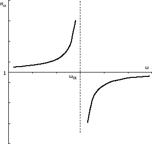
FIGURE 5.9  Normal dispersion.

When the refractive index n_ω increases with frequency ω, as shown in Figure 5.9, the dispersion is called normal. Normal dispersion is caused by the oscillations of electrons and is observed in the entire visible region.

For low frequencies ω ≪ ω_0i, Equation 5.95 assumes the form:

$n=1+\frac{e^2}{2{\text{ε}}_{0}m}{\displaystyle \sum _i\frac{N_i}{{\text{ω}}_{0\text{i}}^2}}$

(5.96)

which gives the static value of the refractive index. As it was discussed above, the static value may differ significantly from the refractive index for optical frequencies.

For very high frequencies such as x-rays, ω ≫ ω_0i, then Equation 5.95 becomes

$n_{\text{ω}}=1-\frac{e^2}{2{\text{ε}}_{0}m{\omega }^2}{\displaystyle \sum _i{N}_i}$

(5.97)

This expression shows that the refractive index tends to, but remains, less than unity. This means that for a radiation of very high frequencies, a dielectric behaves as an optically less dense material than vacuum. The reason for this effect is that at very high frequencies, the nature of the electron bonds in the atom does not play any role, and as per Equation 5.97, the refractive index depends only on the total number of oscillating electrons per unit volume.

5.2.4.3    Anomalous Dispersion

The dispersion Equation 5.94 was derived from Equation 5.92 when γ = 0, that is, the damping of oscillations was not taken into consideration. For this case, the refractive index nω turns to infinity at the resonant frequency ω = ω_0i. If damping of oscillations is not ignored, γ ≠ 0, the dispersion curve becomes continuous in the neighborhood of the natural oscillation frequencies ω_0i and does not turn to infinity at ω = ω_0i. For rare gases, when the refractive index differs slightly from unity, Equation 5.92 can be written as

${\widehat{n}}_{\text{ω}}=\sqrt{{\text{ε}}_{\text{rω}}}=n_{\text{ω}}+i{\text{ξ}}_{\text{ω}}\cong 1+\frac{e^2}{2{\text{ε}}_{0}m}\frac{N}{{\text{ω}}_{0\text{i}}^2-{\text{ω}}^2-i\gamma \text{ω}}$

(5.98)

Writing separately the real and imaginary parts

$n_{\text{ω}}=1+\frac{e^2}{2{\text{ε}}_{0}m}\cdot \frac{N\left({\text{ω}}_0^2-{\text{ω}}^2\right)}{\left({\text{ω}}_{0\text{i}}^2-{\text{ω}}^2\right)+{\gamma }^2{\text{ω}}^2}$

(5.99)

and

${\text{ξ}}_{\text{ω}}=\frac{e^2}{2{\text{ε}}_{0}m}\cdot \frac{N\gamma \text{ω}}{\left({\text{ω}}_{0\text{i}}^2-{\text{ω}}^2\right)+{\gamma }^2{\text{ω}}^2}$

(5.100)

The imaginary part ξω of the refractive index describes the absorption in the material. Equation 5.99 shows that near the resonance frequency ω = ω_0i, the refractive index decreases with increasing frequency. This phenomenon is called anomalous dispersion. Normal dispersion is observed throughout the region where a material is transparent, while anomalous dispersion takes place in the absorption regions.

The electric vector of a plane wave propagating in the direction of the z-axis can be presented as

$E\left(z,t\right)=E_0{\text{e}}^{-i\left(\text{ω}t-kz\right)}=E_0{\text{e}}^{-i{\text{ξ}}_{\text{ω}}z/c}{\text{e}}^{-i\left(\text{ω}t-\text{ω}{n}_{\text{ω}}z/c\right)}$

(5.101)

where the wave vector

$k=\frac{\text{ω}}{v}=\text{ω}\frac{\sqrt{{\text{ε}}_{r\text{ω}}}}{c}=\text{ω}\frac{n_{\text{ω}}}{c}+i\text{ω}\frac{{\text{ξ}}_{\text{ω}}}{c}$

(5.102)

was expressed with the complex form of the refractive index from Equation 5.93, ${\widehat{n}}_{\text{ω}}=\sqrt{{\text{ε}}_{r\text{ω}}}=n_{\text{ω}}+i{\text{ξ}}_{\text{ω}}$. Equation 5.101 shows that due to absorption (γ ≠ 0) in the material, the amplitude of the wave decreases exponentially with the traveled distance in the medium, that is, the imaginary part ξ_ω of the refractive index describes the damping of a plane wave in a dielectric. At frequencies near the resonance frequencies ω = ω_0i, the wave energy is consumed, on exciting forced oscillations in electrons. In turn, the oscillating electrons reemit EM waves of the same frequencies but in random directions. This results in scattering of the EM waves upon passing through a dielectric. The scattering is insignificant when γ is small.

5.2.4.4    Group Velocity of a Wave Packet

A wave packet or a pulse, is a superposition of waves whose frequencies and wave numbers are confined to a quite narrow interval. A wave packet of waves with the same polarization can be represented in the form:

$E\left(z,t\right)=\frac{1}{2\pi }{\displaystyle \underset{-\infty }{\overset{+\infty }{\int }}F\left(k\right){\text{e}}^{-i\left(\text{ω}t-kz\right)}}\text{d}k$

(5.103)

The amplitude F(k) describes the distribution of the waves over wave number and hence over frequencies. Thus, F(k) is the Fourier transform of E(z,0) at t = 0:

$F\left(k\right)={\displaystyle \underset{-\infty }{\overset{+\infty }{\int }}E\left(z,0\right)e^{-ikz}dz}$

(5.104)

The amplitude of the wave packet is nonzero only in the narrow interval of values of k near k₀ and has a sharp peak near k₀. Usually, when we speak of the velocity of a signal, we mean the group velocity at a frequency corresponding to the maximum amplitude in the signal. The shape of the pulse does not change when the pulse moves with a group velocity:

$v_g=\frac{{\text{dω}}_0}{\text{d}{k}_0}=\frac{\text{d}\left[2\pi c/\left(n\lambda \right)\right]}{\text{d}\left(2\pi /\lambda \right)}=c\frac{\left(n\text{d}\lambda \text{+}\lambda \text{d}n\right)}{\text{d}\lambda /{\lambda }^2}=\frac{c}{n}\left(1+\frac{\lambda }{n}\frac{\text{d}n}{\text{d}\lambda }\right)$

(5.105)

It is obvious that the group velocity of the pulse depends on the degree of monochromaticity of the wave packet.

5.2.4.5    Color of Objects

The coloration of bodies results from the selective absorption of light at the resonance frequencies ω_0i. When the natural oscillation frequencies ω_0i lie in the UV region, the materials appear almost colorless and transparent, because there is no absorption in the visible part of the spectrum. For example, glass is transparent for wavelengths in the visible range, but strongly absorbs UV. The absorption may occur in the bulk of a body or in its surface layer. When light is reflected from a surface, the most strongly reflected wavelengths are those which are absorbed most strongly upon passing through the bulk of the material. The color due to selective reflection and the color due to selective absorption are complementary (added together they produce white light). For example, a chunk of gold has a reddish-yellow color due to selective reflection. However, a very thin foil of gold exhibits a deep blue color when viewed through, which is due to selective absorption.

5.2.5    PROPAGATION OF LIGHT IN METAMATERIALS

MMs are artificially constructed materials or composites that exhibit negative index of refraction [50,51,53]. MMs are also called negative-index materials, double negative media, backward media, left-handed materials, or negative phase-velocity (NPV) materials, the last being the least ambiguous of all suggested names. First reported in 2000 [50], MMs are the most recent example of a qualitatively new type of material. In comparison with their constituent materials, MMs have distinct and possibly superior properties. Their exotic properties and potential for unusual applications in optics, photonics, electromagnetism, material science, and engineering have garnered significant scientific interest and provide the rationale for ongoing investigation of this rapidly evolving field. The MMs comprise an array of subwavelength-discrete and subwavelength-independent elements designed to respond preferentially to the electric or magnetic component of an external EM wave. Thus, they have a remarkable potential to control EM radiation.

Already in 1968, on the base of theoretical considerations, Veselago predicted many unusual properties of substances with simultaneously negative real permittivity and negative real permeability, including inverse refraction, negative radiation pressure (change from radiation pressure to radiation tension), and inverse Doppler effect [54]. But it was the first observation of the negative refraction by Smith et al. [50] in 2000 that made the breakthrough and initiated intensive research in this area. The phenomenon was first demonstrated with a composite medium, based on a periodic array of interspaced conducting nonmagnetic split ring resonators and continuous wires that exhibit simultaneously negative values of effective permittivity and permeability in the microwave frequency region. The current implementations of negative refractive index media have occurred at microwave to near-optical frequencies (from about 10 GHz to about 100 THz) and in a narrow frequency band [55,56,57]. The extension of MMs to the visible range and the implementation of structures with tunable and reconfigurable resonant properties would be significant for at least two reasons: the opportunity to study and begin to understand the intrinsic properties of negative media and possible future applicability [5859,60,61,62,63,64]. MMs, although fabricated with a microstructure, are effectively homogenous in the frequency range wherein negative refraction is observed. Negative refraction by periodically inhomogeneous substances such as photonic crystals has also been demonstrated theoretically as well as experimentally. Some composite media with simple structure, consisting of insulating magnetic spherical particles embedded in a background matrix, can also exhibit negative permeability and permittivity over significant bandwidths [64]. Due to some practical difficulties in achieving negative refraction in isotropic dielectric–magnetic materials, attention has been directed toward more complex materials such as anisotropic materials [65] as well as isotropic chiral materials [66,67,68,69].

The phase velocity of light propagating in materials with real relative permittivity and real relative permeability both being simultaneously negative is negative. The phase velocity of an EM wave is described as negative, if it is directed opposite to the power flow given by the time-averaged Poynting vector. Negative phase velocity results in negative refraction, which is shown in Figure 5.10. This phenomenon does not contradict Snell’s law. A comprehensive theoretical description of propagation of light in isotropic NPV materials is presented in a series of works of Lakhtakia: for example, propagation of plane wave in a linear, homogeneous, isotropic, and dielectric–magnetic medium [60,67,69,70,71,72,72]; propagation of a plane wave in anisotropic chiral materials [66,73]; and diffraction of a plane wave from periodically corrugated boundary of vacuum and a linear, homogeneous, uniaxial, and dielectric–magnetic NPV medium [67,74]. The study of diffraction from a NPV medium is especially important, because all experimental realizations of NPV MMs so far are based on periodical structures of composite materials, with size of the unit cell smaller than the wavelength. On another hand, gratings made of NPV materials offer quite different properties from the traditional gratings.

The two material parameters that govern the response of homogeneous media to external EM field are the permittivity ε and the magnetic permeability μ. In dielectrics, the role of permeability is ignored. For NPV MMs though, the permeability is of the same importance as the permittivity. In general, both ε and μ are frequency-dependent complex quantities, given by

$\text{ε}\left(\text{ω}\right)={\text{ε}}^{\prime }\left(\text{ω}\right)+i{\text{ε}}^{″}\left(\text{ω}\right)$

(5.106a)

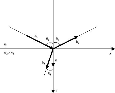
FIGURE 5.10  Negative refraction at a boundary between two isotropic media (n₂> n₁).

and

$\text{μ}\left(\text{ω}\right)={\text{μ}}^{\prime }\left(\text{ω}\right)+i{\text{μ}}^{″}\left(\text{ω}\right)$

(5.106b)

Thus, there are in total four parameters that completely describe the response of an isotropic material to EM radiation at a given frequency.

The theoretical description of negative refraction is out of the scope of this chapter. Moreover, there is no universal model that would fit the description of all particular cases of microstructures that have been observed to exhibit negative refraction. However, let us briefly discuss here as an example, the particular case of total internal reflection when the optically rarer medium has negative real permittivity and negative real permeability, as presented by Lakhtakia [72]. Consider a planar interface of two homogeneous media with relative permittivity ε₁ and ε₂, and relative permeability μ₁ and μ₂, respectively, defined by Equations 106a and b at a given angular frequency ω. The first medium is non-dissipative (${{\text{ε}}^{″}}_1=0$ and ${{\text{μ}}^{″}}_1=0$), while dissipation in the second medium is very small (${{\text{ε}}^{″}}_1\ll {{\text{ε}}^{\prime }}_2$ and ${{\text{μ}}^{″}}_2\ll {{\text{μ}}^{\prime }}_2$). A plane wave is incident on the interface through the first medium and reflected back. The amplitude reflection coefficients in this case are given by

$r_{\left|\right|}=\frac{1-\left({\alpha }_1/{\alpha }_2\right)\left({\text{ε}}_2/{\text{ε}}_1\right)}{1+\left({\alpha }_1/{\alpha }_2\right)\left({\text{ε}}_2/{\text{ε}}_1\right)}$

(5.107a)

for electric vector oscillating in the plane of incidence, and

$r_{\perp }=-\frac{1-\left({\alpha }_1/{\alpha }_2\right)\left({\text{μ}}_2/{\text{μ}}_1\right)}{1+\left({\alpha }_1/{\alpha }_2\right)\left({\text{μ}}_2/{\text{μ}}_1\right)}$

(5.107b)

for perpendicular polarization. In these equations,

$\begin{array}{ccc}{\alpha }_1=k_0\sqrt{{\epsilon }_1{\mu }_1-{\epsilon }_1{\mu }_1{\sin }^2{\theta }_{\text{i}}}& \text{and}& {\alpha }_2=k_0\sqrt{{\epsilon }_2{\mu }_2-{\epsilon }_1{\mu }_1{\sin }^2{\theta }_{\text{i}}}\end{array}$

(5.108)

where

k₀ is the free-space wave number

θ_i is the angle of incidence

The second medium must be a passive medium, thus the imaginary part of α₂ must be positive or equal to zero.

For the phase velocity to oppose the direction of the time-averaged Poynting vector, the inequality

$\left(\left|{\text{ε}}_2\right|-{\text{ε}}_2^{\prime }\right)\left(\left|{\text{μ}}_2\right|-{\text{μ}}_2^{\prime }\right)>{\text{ε}}_2^{″}{\text{μ}}_2^{″}$

(5.109)

has to be satisfied. Thus arises the conclusion that both ${{\epsilon }^{\prime }}_2$ and ${{\mu }^{\prime }}_2$ do not have to be simultaneously negative for the phase velocity to be negative [72].

Total internal reflection occurs at angles of incidence larger than the critical angle. In dielectrics, where only permittivity plays a role, the Goos–Hänchen shift is positive, as shown in Figure 5.7. For NPV materials though, because of equal involvement of permeability and permittivity, the reversal of the signs of both results in a reversal of the direction of the Goos–Hänchen shift. Figure 5.11 shows a negative Goos–Hänchen shift. Furthermore, if both the real permittivity and the real permeability of the optically rarer medium are negative, the negative Goos–Hänchen shifts occur for both perpendicular and parallel polarized beams [72].

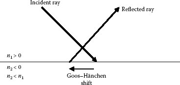
FIGURE 5.11  Negative Goos–Hänchen shift on total reflection. (After Lakhtakia, A., Int. J. Electron. Commun., 58, 229, 2004.)

The area of artificial MMs is a subject of huge scientific interest with exponentially growing number of publications. The brief introduction here is aimed to provide some initial information for those who might be interested in expanding their knowledge in this direction.

REFERENCES

1.  Born, M. and Wolf, E., Principles of Optics, 6th edn., Pergamon Press, New York, 1980.

2.  Matveev, A.N., Optics, Mir Publishers, Moscow, Russia, 1988.

3.  Smith, F.G., King, T.A., and Wilkins, D., Optics and Photonics, 2nd edn., John Wiley & Sons, Inc., Hoboken, NJ, 2007.

4.  Hecht, E., Optics, 4th edn., Pearson Education, Inc., Addison Wesley, San Francisco, CA, 2002.

5.  Bennett, C.A., Principles of Physical Optics, John Wiley & Sons, Inc., Hoboken, NJ, 2008.

6.  Pedrotti, F.L., Pedrotti, L.S., and Pedrotti L.M., Introduction to Optics, 3rd edn., Pearson Prentice Hall, Upper Saddle River, NJ, 2007, p. 421.

7.  Möller, K.D., Optics, University Science Books, Mill Valley, CA, 1988, p. 384.

8.  Klein, M.V. and Furtak, T.E., Optics, 2nd edn., John Wiley & Sons, Inc., Hoboken, NJ, 1986, p. 475.

9.  Strong, J., Concepts of Classical Optics, W.H. Freeman and Co., San Francisco, CA, 1958; or Dover Publications, New York, 2004.

10.  Halliday, D., Resnick, R.P., and Walker, J., Fundamentals of Physics, 7th edn., John Wiley & Sons, Hoboken, NJ, 2004.

11.  Fowles, G.R., Introduction to Modern Optics, 2nd edn., Dover Publications, New York, 1989.

12.  Guenther, R.D., Modern Optics, John Wiley & Sons, Hoboken, NJ, 1990.

13.  Saleh, B.E.A. and Teich, M.C., Fundamentals of Photonics, 2nd edn., John Wiley & Sons, Inc., Hoboken, NJ, 2007.

14.  Meyer-Arendt, J.R., Introduction to Classical and Modern Optics, 4th edn., Prentice-Hall, Inc., Englewood Cliffs, NJ, 1995.

15.  Scully, M.O. and Zubairy, M.S., Quantum Optics, Cambridge University Press, Cambridge, U.K., 1997.

16.  Griffithz, D.J., Introduction to Electrodynamics, 3rd edn., Prentice-Hall, Inc., Englewood Cliffs, NJ, 1999.

17.  Jackson, J.D., Classical Electrodynamics, 3rd edn., John Wiley & Sons, Inc., New York, 1998.

18.  Grant, I.S. and Phillips, W.R., Electromagnetism, 2nd edn., John Wiley & Sons, Inc., New York, 1990.

19.  Boas, M.L., Mathematical Methods in the Physical Sciences, 3rd edn., John Wiley & Sons, Inc., Hoboken, NJ, 2006.

20.  Shen, Y.R., The Principles of Nonlinear Optics, John Wiley & Sons, Inc., New York, 1984.

21.  Boyd, R.W., Nonlinear Optics, 2nd edn., Academic Press, London, U.K., 2003.

22.  Sheik-Bahae, M. et al., Sensitive measurement of optical nonlinearities using a single beam, IEEE Journal of Quantum Electronics 26, 760, 1990.

23.  Balu, M. et al., White-light continuum Z-scan technique for nonlinear materials characterization, Optics Express 12, 3820, 2004.

24.  Dushkina, N.M. et al., Influence of the crystal direction on the optical properties of thin CdS films formed by laser ablation, Photodetectors: Materials and Devices IV, San Jose, CA; Proceedings of SPIE 3629, 424, 1999.

25.  Hariharan, P., Optical Holography, Principles, Techniques, and Applications, 2nd edn., Cambridge University Press, Cambridge, U.K., 1996.

26.  Splinter, R. and Hooper B.A., An Introduction to Biomedical Optics, Taylor & Francis Group, LLC, New York, 2007.

27.  Novotny, L. and Hecht, B., Principles of Nano-Optics, Cambridge University Press, Cambridge, U.K., 2006.

28.  de Fornel, F., Evanescent Waves, Springer, Berlin, Germany, 2001.

29.  Zhu, S. et al., Frustrated total internal reflection: A demonstration and review, American Journal of Physics 54, 601–607, 1986.

30.  Lotsch, H.K.V., Beam displacement at total reflection. The Goos-Hänchen effect I, Optik 32, 116–137, 1970.

31.  Otto, A., Excitation of nonradiative surface plasma waves in silver by the method of frustrated total reflection, Zeitschrift für Physik 216, 398, 1968.

32.  Raether, H., Surface plasma oscillations and their applications, in: Physics of Thin Films, Advances in Research and Development, G. Hass, M.H. Francombe, and R.W. Hofman (Eds.), Vol. 9, Academic Press, New York, 1977, pp. 145–261.

33.  Ehler, T.T. and Noe, L.J., Surface plasmon studies of thin silver/gold bimetallic films, Langmuir 11(10), 4177–4179, 1995.

34.  Homola, J., Yee, S.S., and Gauglitz, G., Surface plasmon resonance sensors: Review, Sensors and Actuators B 54, 3, 1999.

35.  Mulvaney, P., Surface plasmon spectroscopy of nanosized metal particles, Langmuir 12, 788, 1996.

36.  Klar, T. et al., Surface plasmon resonances in single metallic nanoparticles, Physical Review Letters 80, 4249, 1998.

37.  Markel, V.A. et al., Near-field optical spectroscopy of individual surface-plasmon modes in colloid clusters, Physical Review B 59, 10903, 1999.

38.  Kotsev, S.N. et al., Refractive index of transparent nanoparticle films measured by surface plasmon microscopy, Colloid and Polymer Science 281, 343, 2003.

39.  Dushkina, N. and Sainov, S., Diffraction efficiency of binary metal gratings working in total internal reflection, Journal of Modern Optics 39, 173, 1992.

40.  Dushkina, N.M. et al., Reflection properties of thin CdS films formed by laser ablation, Thin Solid Films 360, 222, 2000.

41.  Schuck, P., Use of surface plasmon resonance to probe the equilibrium and dynamic aspects of interactions between biological macromolecules, Annual Review of Biophysics and Biomolecular Structure 26, 541–566, 1997.

42.  Dushkin, C.D. et al., Effect of growth conditions on the structure of two-dimensional latex crystals: Experiment, Colloid and Polymer Science 227, 914–930, 1999.

43.  Tourillon, G. et al., Total internal reflection sum-frequency generation spectroscopy and dense gold nanoparticles monolayer: A route for probing adsorbed molecules, Nanotechnology 18, 415301, 2007.

44.  He, L. et al., Colloidal Au-enhanced surface plasmon resonance for ultrasensitive detection of DNA hybridization, Journal of the American Chemical Society 122, 9071–9077, 2000.

45.  Krenn, J.R. et al., Direct observation of localized surface plasmon coupling, Physical Review B 60, 5029–5033, 1999.

46.  Liebsch, A., Surface plasmon dispersion of Ag, Physical Review Letters 71, 145–148, 1993.

47.  Prieve, D.C. and Frej, N.A., Total internal reflection microscopy: A quantitative tool for the measurement of colloidal forces, Langmuir 6, 396–403, 1990.

48.  Perner, M. et al., Optically induced damping of the surface plasmon resonance in gold colloids, Physical Review Letters 78, 2192–2195, 1993.

49.  Tsuei, K.-D., Plummer, E.W., and Feibelman, P.J., Surface plasmon dispersion in simple metals, Physical Review Letters 63, 2256–2259, 1989.

50.  Smith, D.R. et al., Composite medium with simultaneously negative permeability and permittivity, Physical Review Letters 84, 4184–4187, 2000.

51.  Smith, D.R., Pendry, J.B., and Wiltshire, M.C.K., Metamaterials and negative refractive index, Science 305, 788, 2006.

52.  Lakhtakia, A., McCall, M.W., and Weiglhofer, W.S., Negative phase-velocity mediums, in: Introduction to Complex Mediums for Optics and Electromagnetics, Weiglhofer, W.S. and Lakhtakia, A. (Eds.), SPIE Press, Bellingham, WA, 2003, pp. 347–363.

53.  Ramakrishna, S.A., Physics of negative refractive index materials, Reports on Progress in Physics 68, 449–521, 2005.

54.  Veselago, V.G., The electrodynamics of substances with simultaneously negative values of ε and μ, Soviet Physics Uspekhi 10, 509–514, 1968.

55.  Shelby, R.A., Smith, D.R., and Schultz, S., Experimental verification of a negative index of refraction, Science 292, 77–79, 2001.

56.  Grbic, A. and Eleftheriades, G.V., Experimental verification of backward-wave radiation from a negative index metamaterial, Journal of Applied Physics 92, 5930–5935, 2002.

57.  Houck, A.A., Brock, J.B., and Chuang, I.L., Experimental observations of a left-handed material that obeys Snell’s law, Physical Review Letters 90, 137401, 2003.

58.  Padilla, W.J., Basov, D.N., and Smith, D.R., Negative refractive index metamaterials, Materials Today 9, 28, 2006.

59.  Shalaev, V.M. and Boardman, A. Focus issue on metamaterials, Journal of Optical Society of America B 23, 386–387, 2006.

60.  McCall, M.W., Lakhtakia, A., and Weiglhofer, W.S., The negative index of refraction demystified, European Journal of Physics 23, 353, 2002.

61.  Lakhtakia, A. and McCall, M.W., Focus on negative refraction, New Journal of Physics 7, 191–193, 2005.

62.  Enkrich, C. et al., Magnetic metamaterials at telecommunication and visible frequencies, Physical Review Letters 95, 203901, 2005.

63.  Pendry, J.B., Negative refraction, Contemporary Physics 45, 191–202, 2004.

64.  Holloway, C.L. et al., A double negative (DNG) composite medium composed of magnetodielectric spherical particles embedded in a matrix, IEEE Transactions on Antennas and Propagation 51, 2596, 2003.

65.  Hu, L. and Lin, Z., Imaging properties of uniaxially anisotropic negative refractive index materials, Physics Letters A 313, 316–324, 2003.

66.  Mackay, T.G. and Lakhtakia, A., Plane waves with negative phase velocity in Faraday chiral mediums, Physical Review E 69, 026602, 2004.

67.  Lakhtakia, A., Reversed circular dichroism of isotropic chiral mediums with negative real permeability and permittivity, Microwave and Optical Technology Letters 33, 96–97, 2002.

68.  Pendry, J.B., A chiral route to negative refraction, Science 306, 1353–1355, 2004.

69.  Mackay, T.G., Plane waves with negative phase velocity in isotropic mediums, Microwave and Optical Technology Letters 45, 120–121, 2005; a corrected version is available at: http://www.arxiv.org/abs/physics/0412131.

70.  Lakhtakia, A. and Mackay, T.G., Fresnel coefficients for a permittivity-permeability phase space encompassing vacuum, anti-vacuum, and nihility, Microwave and Optical Technology Letters 48, 265–270, 2006.

71.  Lakhtakia, A., On planewave remittances and Goos-Hänchen shifts on planar slabs with negative real permittivity and permeability, Electromagnetics 23, 71–75, 2003.

72.  Lakhtakia, A., Positive and negative Goos-Hänchen shifts and negative phase-velocity mediums (alias left-handed materials), International Journal of Electronics and Communications (AEÜ) 58, 229–231, 2004.

73.  Mackay, T.G. and Lakhtakia, A., Negative phase velocity in a material with simultaneous mirror-conjugated and racemic chirality characteristics, New Journal of Physics 7(165), 1–23, 2005.

74.  Depine, R.A. and Lakhtakia, A., Diffraction by a grating made of a uniaxial dielectric-magnetic medium exhibiting negative refraction, New Journal of Physics 7, 1–23, 2005.