Day 24. Advanced OSPFv2 and OSPFv3
ENCOR 350-401 Exam Topics
• Infrastructure
• Configure and verify simple OSPF environments, including multiple normal areas, summarization, and filtering (neighbor adjacency, point-to-point and broadcast network types, and passive interface)
Key Topics
Today we review advanced OSPFv2 optimization features, such as OSPF cost manipulation, route filtering, summarization, and default routing. We also look at OSPFv3 configuration and tuning using the newer address family (AF) framework that supports IPv4 and IPv6.
OSPF Cost
A metric is an indication of the overhead required to send packets across a certain interface. OSPF uses cost as a metric. A smaller cost indicates a better path than a higher cost. By default, on Cisco devices, the cost of an interface is inversely proportional to the bandwidth of the interface, so a higher bandwidth has a lower OSPF cost since it takes longer for packets to cross a 10 Mbps link than a 1 Gbps link.
The formula that you use to calculate OSPF cost is:
The default reference bandwidth is 108, which is 100,000,000. This is equivalent to the bandwidth of a Fast Ethernet interface. Therefore, the default cost of a 10-Mbps Ethernet link is 108 / 107 = 10, and the cost of a 100 Mbps link is 108 / 108 = 1.
A problem arises with links that are faster than 100 Mbps. Because the OSPF cost has to be a positive integer, all links that are faster than Fast Ethernet have an OSPF cost of 1. Since most networks today are operating with faster speeds, it may be a good idea to consider changing the default reference bandwidth value on all routers within an AS. However, you need to be aware of the consequences of making such changes. Because the link cost is a 16-bit number, increasing the reference bandwidth to differentiate between high-speed links might result in a loss of differentiation in your low speed links. The 16-bit value provides OSPF with a maximum cost value of 65,535 for a single link. If the reference bandwidth were changed to 1011, 100-Gpbs links would have a value of 1, 10-Gpbs links would be 10, and so on. The issue is that for a T1 link, the cost is now 64,766 (1011/1.544 Mbps) and anything slower than that will now have the largest OSPF cost value of 65,535.
To improve OSPF behavior, you can adjust the reference bandwidth to a higher value by using the auto-cost reference-bandwidth OSPF configuration command. Note that this setting is local to each router. If this setting is used, it is recommended that it be applied consistently across the network. You can indirectly set the OSPF cost by configuring the bandwidth speed interface subcommand (where speed is in Kbps). In such cases, the formula shown earlier is used—just with the configured bandwidth value. The most controllable method of configuring OSPF costs, but the most laborious, is to configure the interface cost directly. Using the ip ospf cost interface configuration command, you can directly change the OSPF cost of a specific interface. The cost of the interface can be set to a value between 1 and 65535. This command overrides whatever value is calculated based on the reference bandwidth and the interface bandwidth.
Shortest Path First Algorithm
The shortest path first (SPF), or Dijkstra, algorithm places each router at the root of the OSPF tree and then calculates the shortest path to each node. The path calculation is based on the cumulative cost that is required to reach that destination. For example, in Figure 24-1, R1 has calculated a total cost of 30 to reach the R4 LAN via R2 and a total of 40 to reach the same LAN via R3. The path with a cost of 30 will be chosen as the best path in this case because a lower cost is better.

Figure 24-1 OSPF Cost Calculation Example
Link-state advertisements (LSAs) are flooded throughout the area using a reliable process, which ensures that all the routers in an area have the same topological database. Each router uses the information in its topological database to calculate a shortest path tree, with itself as the root. The router then uses this tree to route network traffic.
Figure 24-2 shows the R1 view of the network, where R1 is the root and calculates the pathways to every other device based on itself as the root. Keep in mind that each router has its own view of the topology, even though all the routers build the shortest path trees by using the same link-state database.

Figure 24-2 OSPF SPF Tree
LSAs are flooded through the area in a reliable manner with OSPF, which ensures that all routers in an area have the same topological database. Because of the flooding process, R1 has learned the link-state information for each router in its routing area. Each router uses the information in its topological database to calculate a shortest path tree with itself as the root. The tree is then used to populate the IP routing table with the best paths to each network.
For R1, the shortest path to each LAN and its cost are shown in Figure 24-2. The shortest path is not necessarily the best path. Each router has its own view of the topology, even though the routers build shortest path trees by using the same link-state database. Unlike with EIGRP, when OSPF determines the shortest path based on all possible paths, it discards any information pertaining to these alternate paths. Any paths not marked as “shortest” would be trimmed from the SPF tree list. During a topology change, the Dijkstra algorithm is run to recalculate the shortest paths for any affected subnets.
OSPF Passive Interfaces
Passive interface configuration is a common method for hardening routing protocols and reducing the use of resources. It is also supported by OSPF.
Use the passive-interface default router configuration command to enable this feature for all interfaces or use the passive-interface interface-id router configuration command to make specific interfaces passive.
When you configure a passive interface under the OSPF process, the router stops sending and receiving OSPF hello packets on the selected interface. Use passive interface configuration only on interfaces where you do not expect the router to form any OSPF neighbor adjacency. When you use the passive interface setting as default, you can identify interfaces that should remain active with the no passive-interface configuration command.
OSPF Default Routing
To be able to perform routing from an OSPF domain toward external networks or toward the Internet, you must either know all the destination networks or create a default route noted as 0.0.0.0/0.
The default routes provide the most scalable approach. Default routing guarantees smaller routing tables and ensures that fewer resources are consumed on the routers. There is no need to recalculate the SPF algorithm if one or more networks fail.
To implementing default routing in OSPF, you can inject a default route using a type 5 AS external LSA. You implement this by using the default-information originate command on the uplink ASBR, as shown in Figure 24-3. The uplink ASBR connects the OSPF domain to the upstream router in the SP network. The uplink ASBR generates a default route using a type 5 AS external LSA, which is flooded in all OSPF areas except the stub areas.
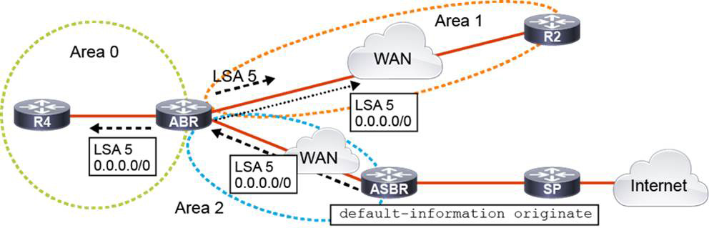
Figure 24-3 OSPF Default Routing
You can use different keywords in the configuration command. To advertise 0.0.0.0/0 regardless of whether the advertising router already has a default route in its own routing table, add the keyword always to the default-information originate command, as shown in this example:
ASBR(config-router)# default-information originate ?
  always       Always advertise default route
  metric       OSPF default metric
  metric-type  OSPF metric type for default routes
  route-map    Route-map reference
<cr>
The router participating in an OSPF network automatically becomes an ASBR when you use the default-information originate command. You can also use a route map to define dependency on any condition inside the route map. The metric and metric-type options allow you to specify the OSPF cost and metric type of the injected default route.
After you configure the ASBR to advertise a default route into OSPF, all other routers in the topology should receive it. Example 24-1 shows the routing table on R4 from Figure 24-3. Notice that R4 lists the default route as an O* E2 route in the routing table because it is learned through a type 5 AS external LSA.
Example 24-1 Verifying the Routing Table on R4
R4# show ip route ospf
<. . . output omitted . . .>

Gateway of last resort is 172.16.25.2 to network 0.0.0.0

O*E2  0.0.0.0/0 [110/1] via 172.16.25.2, 00:13:28, GigabitEthernet0/0
<. . . output omitted . . .>
OSPF Route Summarization
In large internetworks, hundreds or even thousands of network addresses can exist. It is often problematic for routers to maintain this volume of routes in their routing tables. Route summarization, also called route aggregation, is the process of advertising a contiguous set of addresses as a single address with a less specific, shorter subnet mask. This method can reduce the number of routes that a router must maintain because it represents a series of networks as a single summary address.
OSPF route summarization helps solve two major problems: large routing tables and frequent LSA flooding throughout the AS. Every time a route disappears in one area, routers in other areas also get involved in shortest path calculation. To reduce the size of the area database, you can configure summarization on an area boundary or AS boundary.
Normally, type 1 and type 2 LSAs are generated inside each area and translated into type 3 LSAs in other areas. With route summarization, the ABRs or ASBRs consolidate multiple routes into a single advertisement. ABRs summarize type 3 LSAs, and ASBRs summarize type 5 LSAs, as illustrated in Figure 24-4. Instead of advertising many specific prefixes, they advertise only one summary prefix.

Figure 24-4 OSPF Summarization on ABRs and ASBRs
If an OSPF design includes multiple ABRs or ASBRs between areas, suboptimal routing is possible. This behavior is one of the drawbacks of summarization.
Route summarization requires a good addressing plan with an assignment of subnets and addresses that lends itself to aggregation at the OSPF area borders. When you summarize routes on a router, it is possible that OSPF still might prefer a different path for a specific network with a longer prefix match than the one proposed by the summary. Also, the summary route has a single metric to represent the collection of routes summarized. This is usually the smallest metric associated with an LSA included in the summary.
Route summarization directly affects the amount of bandwidth, CPU power, and memory resources the OSPF routing process consumes. Route summarization minimizes the number of routing table entries, localizes the impact of a topology change, and reduce LSA flooding and saves CPU resources. Without route summarization, every specific-link LSA is propagated into the OSPF backbone and beyond, causing unnecessary network traffic and router overhead, as illustrated in Figure 24-5, where a LAN interface in Area 1 has failed. This triggers a flooding of type 3 LSAs throughout the OSPF domain.

Figure 24-5 OSPF Type 3 LSA Flooding
With route summarization, only the summarized routes are propagated into the backbone (Area 0). Summarization prevents every router from having to rerun the SPF algorithm, increases the stability of the network, and reduces unnecessary LSA flooding. Also, if a network link fails, the topology change is not propagated into the backbone (and other areas, by way of the backbone). Specific-link LSA flooding outside the area does not occur.
OSPF ABR Route Summarization
With summarization of type 3 summary LSAs, the router creates a summary of all the interarea (type 1 and type 2 LSAs) routes. It is therefore called interarea route summarization.
To configure route summarization on an ABR, you use the following command:
ABR(config-router)# area area-id range ip-address mask [advertise | not-advertise] [cost cost]
A summary route is advertised only if you have at least one prefix that falls within the summary range. The ABR that creates the summary route creates a Null0 interface to prevent loops. You can configure a static cost for the summary instead of using the lowest metric from one of the prefixes being summarized. The default behavior is to advertise the summary prefix so the advertise keyword is not necessary.
Summarization on an ASBR
It is possible to summarize external networks being advertised by an ASBR. This summarization minimizes the number of routing table entries, reduces type 5 AS external LSA flooding, and saves CPU resources. It also localizes the impact of any topology changes if an external network fails.
To configure route summarization on an ASBR, use the following command:
ASBR(config-router)# summary-address ip-address mask [not-advertise] [tag tag] [nssa-only]
OSPF Summarization Example
Figure 24-6 shows the topology used in this section’s summarization example. The ABR is configured to summarize four prefixes in Area 3, and the ASBR is configured to summarize eight prefixes that originate from the EIGRP external AS.
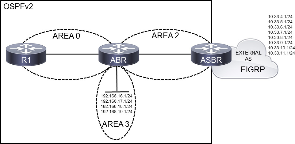
Figure 24-6 OSPF Summarization Topology Example
Example 24-2 shows the routing table on R1 before summarization. Notice that eight external networks (O E2) and four Area 3 networks (O IA) are present.
Example 24-2 Verifying the Routing Table on R1
R1# show ip route ospf
<... output omitted ...>

      10.0.0.0/24 is subnetted, 8 subnets
O E2     10.33.4.0 [110/20] via 172.16.13.2, 01:04:40, GigabitEthernet0/2
O E2     10.33.5.0 [110/20] via 172.16.13.2, 01:04:40, GigabitEthernet0/2
O E2     10.33.6.0 [110/20] via 172.16.13.2, 01:04:40, GigabitEthernet0/2
O E2     10.33.7.0 [110/20] via 172.16.13.2, 01:04:40, GigabitEthernet0/2
O E2     10.33.8.0 [110/20] via 172.16.13.2, 01:04:40, GigabitEthernet0/2
O E2     10.33.9.0 [110/20] via 172.16.13.2, 01:04:40, GigabitEthernet0/2
O E2     10.33.10.0 [110/20] via 172.16.13.2, 01:04:40, GigabitEthernet0/2
O E2     10.33.11.0 [110/20] via 172.16.13.2, 01:04:40, GigabitEthernet0/2
O IA  192.168.16.0/24 [110/11] via 172.16.13.2, 01:04:40, GigabitEthernet0/2
O IA  192.168.17.0/24 [110/11] via 172.16.13.2, 01:04:40, GigabitEthernet0/2
O IA  192.168.18.0/24 [110/11] via 172.16.13.2, 01:04:40, GigabitEthernet0/2
O IA  192.168.19.0/24 [110/11] via 172.16.13.2, 01:04:40, GigabitEthernet0/2
Example 24-3 shows the configuration of summarization on the ABR for the 192.168.16.0/24, 192.168.17.0, 192.168.18.0/24, and 192.168.19.0/24 Area 3 networks into the aggregate route 192.168.16.0/22. Example 24-3 also shows the configuration of summarization on the ASBR for the 10.33.4.0/24 to 10.33.11.0/24 external networks into two aggregate routes, 10.33.4.0/22 and 10.33.8.0/22. Two /22 aggregate routes are used on the ASBR instead of one /21 or one /20 to avoid advertising subnets that don’t exist or that don’t belong in the external AS.
Example 24-3 Configuring Interarea and External Summarization
ABR(config)# router ospf 1
ABR(config-router)# area 3 range 192.168.16.0 255.255.252.0
ASBR(config)# router ospf 1
ASBR(config-router)# summary-address 10.33.4.0 255.255.252.0
ASBR(config-router)# summary-address 10.33.8.0 255.255.252.0
Example 24-4 shows the routing on R1 for verification that the individual longer prefix routes were suppressed and replaced by the interarea route summary (O IA) and the external route summary (O E2).
Example 24-4 Verifying Interarea and External Summarization on R1
R1# show ip route ospf

<... output omitted ...>

      10.0.0.0/22 is subnetted, 2 subnets
O E2     10.33.4.0 [110/20] via 172.16.13.2, 00:11:42, GigabitEthernet0/2
O E2     10.33.8.0 [110/20] via 172.16.13.2, 00:11:42, GigabitEthernet0/2
O IA  192.168.16.0/22 [110/11] via 172.16.13.2, 01:00:15, GigabitEthernet0/2
OSPF Route Filtering Tools
OSPF has built-in mechanisms for controlling route propagation. OSPF routes are permitted or denied into different OSPF areas based on area type. There are several methods to filter routes on the local router, and the appropriate method depends on whether the router is in the same area or in a different area than the originator of the routes. Most filtering methods do not remove the networks from the LSDB. The routes are removed from the routing table, which prevents the local router from using them to forward traffic. The filters have no impact on the presence of routes in the routing table of any other router in the OSPF routing domain.
Distribute Lists
One of the ways to control routing updates is by using a distribute list, which allows you to apply an access list to routing updates. A distribute list filter can be applied to transmitted, received, or redistributed routing updates.
Classic access lists do not affect traffic originated by the router, so applying an access list to an interface has no effect on the outgoing routing advertisements. When you link an access list to a distribute list, routing updates can be controlled no matter what their source.
An access list is configured in global configuration mode and then associated with a distribute list under the routing protocol. An access list should permit the networks that should be advertised or redistributed and deny the networks that should be filtered. The router then applies the access list to the routing updates for that protocol. Options in the distribute-list command allow updates to be filtered based on three factors:
• Incoming interface
• Outgoing interface
• Redistribution from another routing protocol
For OSPF, the distribute-list in command filters what ends up in the IP routing table—and only on the router on which the distribute-list in command is configured. It does not remove routes from the link-state databases of area routers.
It is possible to use a prefix list instead of an access list when matching prefixes for the distribute list. Prefix lists offer better performance than access lists. They can filter based on prefix and prefix length.
Using the ip prefix-list command has several benefits in comparison with using the access-list command. Prefix lists were intended for use with route filtering, whereas access lists were originally intended to be used for packet filtering.
A router transforms a prefix list into a tree structure, and each branch of the tree serves as a test. Cisco IOS Software determines a verdict of either “permit” or “deny” much faster this way than when sequentially interpreting access lists.
You can assign a sequence number to ip prefix-list statements, which gives you the ability to sort statements if necessary. Also, you can add statements at a specific location or delete specific statements. If no sequence number is specified, a default sequence number is applied.
Routers match networks in a routing update against the prefix list by using as many bits as indicated. For example, you can specify a prefix list to be 10.0.0.0/16, which matches 10.0.0.0 routes but not 10.1.0.0 routes.
A prefix list can specify the size of the subnet mask and can also indicate that the subnet mask must be in a specified range.
Prefix lists are similar to access lists in many ways. A prefix list can consist of any number of lines, each of which indicates a test and a result. The router can interpret the lines in the specified order, although Cisco IOS Software optimizes this behavior for processing in a tree structure. When a router evaluates a route against the prefix list, the first line that matches results in either a “permit” or “deny.” If none of the lines in the list match, the result is “implicitly deny.”
Testing is done using IPv4 or IPv6 prefixes. The router compares the indicated number of bits in the prefix with the same number of bits in the network number in the update. If these numbers match, testing continues, with an examination of the number of bits set in the subnet mask. The ip prefix-list command can indicate a prefix length range, and the number must be within that range to pass the test. If you do not indicate a range in the prefix line, the subnet mask must match the prefix size.
OSPF Filtering Options
Internal routing protocol filtering presents some special challenges with link-state routing protocols such as OSPF. Link-state protocols do not advertise routes; instead, they advertise topology information. Also, SPF loop prevention relies on each router in the same area having an identical copy of the LSDB for that area. Filtering or changing LSA contents in transit could conceivably make the LSDBs differ on different routers, causing routing irregularities.
IOS supports four types of OSPF route filtering:
• ABR type 3 summary LSA filtering using the filter-list command: This process prevents an ABR from creating certain type 3 summary LSAs.
• Using the area range not-advertise command: This process also prevents an ABR from creating specific type 3 summary LSAs.
• Filtering routes (not LSAs): With the distribute-list in command, a router can filter the routes that its SPF process is attempting to add to its routing table without affecting the LSDB. This type of filtering can be applied to type 3 summary LSAs and type 5 AS external LSAs.
• Using the summary-address not-advertise command: This command is like the area range not-advertise command but is applied to the ASBR to prevent it from creating specific type 5 AS external LSAs.
OSPF Filtering: Filter List
ABRs do not forward type 1 and type 2 LSAs from one area into another but instead create type 3 summary LSAs for each subnet defined in the type 1 and type 2 LSAs. Type 3 summary LSAs do not contain detailed information about the topology of the originating area; instead, each type 3 summary LSA represents a subnet and a cost from the ABR to that subnet.
The OSPF ABR type 3 summary LSA filtering feature allows an ABR to filter this type of LSAs at the point where the LSAs would normally be created. By filtering at the ABR, before the type 3 summary LSA is injected into another area, the requirement for identical LSDBs inside the area can be met while still filtering LSAs.
To configure this type of filtering, you use the area area-number filter-list prefix prefix-list-name in | out command under OSPF configuration mode. The referenced prefix list is used to match the subnets and masks to be filtered. The area-number and the in | out option of the area filter-list command work together, as follows:
• When out is configured, IOS filters prefixes coming out of the configured area.
• When in is configured, IOS filters prefixes going into the configured area.
Returning to the topology illustrated in Figure 24-6, recall that the ABR is currently configured to advertise a summary of area 3 subnets (192.168.16.0/22). This type 3 summary LSA is flooded into area 0 and area 2. In Example 24-5, the ABR router is configured to filter the 192.168.16.0/22 prefix as it enters area 2. This allows R1 to still receive the summary from area 3, but the ASBR does not.
Example 24-5 Configuring Type 3 Summary LSA Filtering with a Filter List
ABR(config)# ip prefix-list FROM_AREA_3 deny 192.168.16.0/22
ABR(config)# ip prefix-list FROM_AREA_3 permit 0.0.0.0/0 le 32
!
ABR(config)# router ospf 1
ABR(config-router)# area 2 filter-list prefix FROM_AREA_3 in
OSPF Filtering: Area Range
The second way to filter OSPF routes is to filter type 3 summary LSAs at an ABR by using the area range command. The area range command performs route summarization at ABRs, telling a router to cease advertising smaller subnets in a particular address range, instead creating a single type 3 summary LSA whose address and prefix encompass the smaller subnets. When the area range command includes the not-advertise keyword, not only are the smaller component subnets not advertised as type 3 summary LSAs, the summary route is also not advertised. As a result, this command has the same effect as the area filter-list command with the out keyword: It prevents the LSA from going out to any other areas.
Again returning to the topology illustrated in Figure 24-6, instead of using the filter list described previously, Example 24-6 shows the use of the area range command to not only filter out the individual area 3 subnets but also prevent the type 3 summary LSA from being advertised out of area 3.
Example 24-6 Configuring Type 3 Summary LSA Filtering with Area Range
ABR(config)# router ospf 1
ABR(config-router)# area 3 range 192.168.16.0 255.255.252.0 not-advertise
The result here is that neither R1 nor the ASBR receives individual Area 3 prefixes or the summary.
OSPF Filtering: Distribute List
For OSPF, the distribute-list in command filters what ends up in the IP routing table—and only on the router on which the distribute-list in command is configured. It does not remove routes from the link-state database of area routers. The process is straightforward, and the distribute-list command can reference either an ACL or a prefix list.
The following rules govern the use of distribute lists for OSPF:
• The distribute list applied in the inbound direction filters results of SPF (the routes to be installed into the router’s routing table).
• The distribute list applied in the outbound direction applies only to redistributed routes and only on an ASBR; it selects which redistributed routes to advertise. (Redistribution is beyond the scope of this book.)
• The inbound logic does not filter inbound LSAs; it instead filters the routes that SPF chooses to add to its own local routing table.
In Example 24-7, access list number 10 is used as a distribute list and applied in the inbound direction to filter OSPF routes that are being added to its own routing table.
Example 24-7 Configuring a Distribute List with an Access List
R1(config)# access-list 10 deny 192.168.4.0 0.0.0.255
R1(config)# access-list 10 permit any
!
R1(config)# router ospf 1
R1(config-router)# distribute-list 10 in
Example 24-8 shows the use of a prefix list with a distribute list to achieve the same result as with commands in Example 24-7.
Example 24-8 Configuring a Distribute List with a Prefix List
R1(config)# ip prefix-list seq 5 31DAYS-PFL deny 192.168.4.0/24
R1(config)# ip prefix-list seq 10 31DAYS-PFL permit 0.0.0.0/0 le 32
!
R1(config)# router ospf 1
R1(config-router)# distribute-list prefix 31DAYS-PFL in
OSPF Filtering: Summary Address
Recall that type 5 AS external LSAs are originated by an ASBR (router advertising external routes) and flooded through the whole OSPF autonomous system. You cannot limit the way this type of LSA is generated except by controlling the routes advertised into OSPF. When a type 5 AS external LSA is being generated, it uses the RIB contents and honors the summary-address commands if configured.
It is then possible to filter type 5 AS external LSAs on the ASBR in much the same way that type 3 summary LSAs are filtered on the ABR. Using the summary-address not-advertise command allows you to specify which external networks should be flooded across the OSPF domain as type 5 AS external LSAs.
Returning to the topology illustrated in Figure 24-6, recall that the ASBR router is adverting two type 5 AS external LSAs into the OSPF domain: 10.33.4.0/22 and 10.33.8.0/22. Example 24-9 shows the commands used to prevent the 10.33.8.0/22 type 5 summary or the individual subnets that are part of that summary from being advertised into the OSPF domain.
Example 24-9 Configuring Type 5 AS External LSA Filtering
ASBR(config)# router ospf 1
ASBR(config-router)# summary-address 10.33.8.0 255.255.252.0 not-advertise
OSPFv3
While OSPFv2 is feature rich and widely deployed, it does have one major limitation in that it does not support the routing of IPv6 networks. Fortunately, OSPFv3 does support IPv6 routing, and it can be configured to also support IPv4 routing.
The traditional OSPFv2 method, which is configured with the router ospf command, uses IPv4 as the transport mechanism. The legacy OSPFv3 method, which is configured with the ipv6 router ospf command, uses IPv6 as the transport protocol.
The newer OSPFv3 address family framework, which is configured with the router ospfv3 command, uses IPv6 as the transport mechanism for both IPv4 and IPv6 address families. Therefore, it does not peer with routers running the traditional OSPFv2 protocol. The OSPFv3 address family framework utilizes a single OSPFv3 process. It is capable of supporting IPv4 and IPv6 within that single OSPFv3 process. OSPFv3 builds a single database with LSAs that carry IPv4 and IPv6 information. The OSPF adjacencies are established separately for each address family. Settings that are specific to an address family (IPv4/IPv6) are configured inside that address family router configuration mode.
The OSPFv3 address family framework is supported as of Cisco IOS Release 15.1(3)S and Cisco IOS Release 15.2(1)T. Cisco devices that run software older than these releases and third-party devices do not form neighbor relationships with devices running the address family feature for the IPv4 address family because they do not set the address family bit. Therefore, those devices do not participate in the IPv4 address family SPF calculations and do not install the IPv4 OSPFv3 routes in the IPv6 RIB.
Although OSPFv3 is a rewrite of the OSPF protocol to support IPv6, its foundation remains the same as in IPv4 and OSPFv2. The OSPFv3 metric is still based on interface cost. The packet types and neighbor discovery mechanisms are the same in OSPFv3 as they are for OSPFv2, except for the use of IPv6 link-local addresses. OSPFv3 also supports the same interface types, including broadcast and point-to-point. LSAs are still flooded throughout an OSPF domain, and many of the LSA types are the same, although a few have been renamed or newly created.
More recent Cisco routers support both the legacy OSPFv3 commands (ipv6 router ospf) and the newer OSPFv3 address family framework (router ospfv3). The focus of this book is on the latter. Routers that use the legacy OSPFv3 commands should be migrated to the newer commands used in this book. Use the Cisco Feature Navigator (https://cfnng.cisco.com/) to determine compatibility and support.
To start any IPv6 routing protocols, you need to enable IPv6 unicast routing by using the ipv6 unicast-routing command.
The OSPF process for IPv6 no longer requires an IPv4 address for the router ID, but it does require a 32-bit number to be set. You define the router ID by using the router-id command. If you do not set the router ID, the system tries to dynamically choose an ID from the currently active IPv4 addresses. If there are no active IPv4 addresses, the process fails to start.
In the IPv6 router ospfv3 configuration mode, you can specify the passive interfaces (using the passive-interface command), enable summarization, and fine-tune the operation, but there is no network command. Instead, you enable OSPFv3 on interfaces by specifying the address family and the area for that interface to participate in.
The IPv6 address differs from the IPv4 addresses. You have multiple IPv6 interfaces on a single interface: a link-local address and one or more global addresses, among others. OSPF communication within a local segment is based on link-local addresses and not global addresses. These differences are one of the reasons you enable the OSPF process per interface in the interface configuration mode and not with the network command.
To enable the OSPF-for-IPv6 process on an interface and assign that interface to an area, use the ospfv3 process-id [ipv4 | ipv6] area area-id command in interface configuration mode. To be able to enable OSPFv3 on an interface, the interface must be enabled for IPv6. This implementation is typically achieved by configuring a unicast IPv6 address. Alternatively, you could enable IPv6 by using the ipv6 enable interface command, which causes the router to derive its link-local address.
By default, OSPF for IPv6 advertises a /128 prefix length for any loopback interfaces that are advertised into the OSPF domain. The ospfv3 network point-to-point command ensures that a loopback with a /64 prefix is advertised with the correct prefix length (64 bits) instead of a prefix length of 128.
OSPFv3 LSAs
OSPFv3 renames two LSA types and defines two additional LSA types that do not exist in OSPFv2.
These are the two renamed LSA types:
• Interarea prefix LSAs for ABRs (type 3): Type 3 LSAs advertise internal networks to routers in other areas (interarea routes). A type 3 LSA may represent a single network or a set of networks summarized into one advertisement. Only ABRs generate summary LSAs. In OSPFv3, addresses for these LSAs are expressed as prefix/prefix-length instead of address and mask. The default route is expressed as a prefix with length 0.
• Interarea router LSAs for ASBRs (type 4): Type 4 LSAs advertise the location of an ASBR. An ABR originates an interarea router LSA into an area to advertise an ASBR that resides outside the area. The ABR originates a separate interarea router LSA for each ASBR it advertises. Routers that are trying to reach an external network use these advertisements to determine the best path to the next hop toward the ASBR.
These are the two new LSA types:
Link LSAs (type 8): Type 8 LSAs have local-link flooding scope and are never flooded beyond the link with which they are associated. Link LSAs provide the link-local address of the router to all other routers that are attached to the link. They inform other routers that are attached to the link of a list of IPv6 prefixes to associate with the link. In addition, they allow the router to assert a collection of option bits to associate with the network LSA that will be originated for the link.
• Intra-area prefix LSAs (type 9): A router can originate multiple intra-area prefix LSAs for each router or transit network, each with a unique link-state ID. The link-state ID for each intra-area prefix LSA describes its association to either the router LSA or the network LSA. The link-state ID also contains prefixes for stub and transit networks.
OSPFv3 Configuration
Figure 24-7 shows a simple four-router topology to demonstrate multiarea OSPFv3 configuration. An OSPFv3 process can be configured to be IPv4 or IPv6. The address-family command is used to determine which AF runs in the OSPFv3 process. Once the address family is selected, you can enable multiple instances on a link and enable address family–specific commands. Loopback 0 is configured as passive under the IPv4 and IPv6 address families. The Loopback 0 interface is also configured with the OSPF point-to-point network type to ensure that OSPF advertises the correct prefix length (/24 for IPv4 and /64 for IPv6). A router ID is also manually configured for the entire OSPFv3 process on each router. R2 is configured to summarize the 2001:db8:0:4::/64 and 2001:db8:0:5::/64 IPv6 prefixes that are configured on R4’s Loopback 0 interface. Finally, R2 is configured with a higher OSPF priority to ensure that it is chosen as the DR on all links. Example 24-10 demonstrates the necessary configuration.
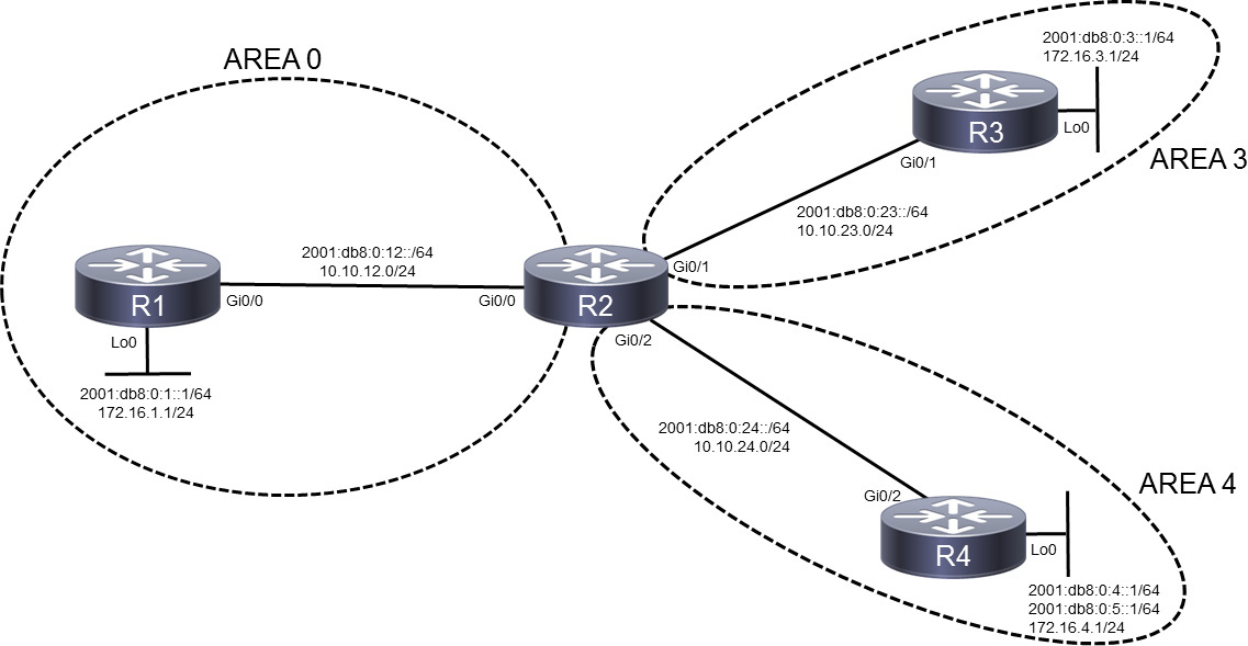
Figure 24-7 Multiarea OSPFv3 Configuration
Example 24-10 Configuring OSPFv3 for IPv4 and IPv6
R1
interface Loopback0
 ip address 172.16.1.1 255.255.255.0
 ipv6 address 2001:DB8:0:1::1/64
 ospfv3 network point-to-point
 ospfv3 1 ipv6 area 0
 ospfv3 1 ipv4 area 0
!
interface Ethernet0/0
 ip address 10.10.12.1 255.255.255.0
 ipv6 address 2001:DB8:0:12::1/64
 ospfv3 1 ipv6 area 0
 ospfv3 1 ipv4 area 0
!
router ospfv3 1
 router-id 1.1.1.1
 !
 address-family ipv4 unicast
  passive-interface Loopback0
 exit-address-family
 !
 address-family ipv6 unicast
  passive-interface Loopback0
 exit-address-family
R2
interface Ethernet0/0
 ip address 10.10.12.2 255.255.255.0
 ipv6 address 2001:DB8:0:12::2/64
 ospfv3 priority 2
 ospfv3 1 ipv6 area 0
 ospfv3 1 ipv4 area 0
!
interface Ethernet0/1
 ip address 10.10.23.1 255.255.255.0
 ipv6 address 2001:DB8:0:23::1/64
 ospfv3 priority 2
 ospfv3 1 ipv4 area 3
 ospfv3 1 ipv6 area 3
!
interface Ethernet0/2
 ip address 10.10.24.1 255.255.255.0
 ipv6 address 2001:DB8:0:24::1/64
 ospfv3 priority 2
 ospfv3 1 ipv6 area 4
 ospfv3 1 ipv4 area 4
!
router ospfv3 1
 router-id 2.2.2.2
 !
 address-family ipv4 unicast
 exit-address-family
 !
 address-family ipv6 unicast
  area 4 range 2001:DB8:0:4::/63
 exit-address-family
R3
interface Loopback0
 ip address 172.16.3.1 255.255.255.0
 ipv6 address 2001:DB8:0:3::1/64
 ospfv3 network point-to-point
 ospfv3 1 ipv6 area 3
 ospfv3 1 ipv4 area 3
!
interface Ethernet0/1
 ip address 10.10.23.2 255.255.255.0
 ipv6 address 2001:DB8:0:23::2/64
 ospfv3 1 ipv6 area 3
 ospfv3 1 ipv4 area 3
!
router ospfv3 1
 router-id 3.3.3.3
 !
 address-family ipv4 unicast
  passive-interface Loopback0
 exit-address-family
 !
 address-family ipv6 unicast
  passive-interface Loopback0
 exit-address-family
R4
interface Loopback0
 ip address 172.16.4.1 255.255.255.0
 ipv6 address 2001:DB8:0:4::1/64
 ipv6 address 2001:DB8:0:5::1/64
 ospfv3 network point-to-point
 ospfv3 1 ipv6 area 4
 ospfv3 1 ipv4 area 4
!
interface Ethernet0/2
 ip address 10.10.24.2 255.255.255.0
 ipv6 address 2001:DB8:0:24::2/64
 ospfv3 1 ipv6 area 4
 ospfv3 1 ipv4 area 4
!
router ospfv3 1
 router-id 4.4.4.4
 !
 address-family ipv4 unicast
  passive-interface Loopback0
 exit-address-family
 !
 address-family ipv6 unicast
  passive-interface Loopback0
 exit-address-family
In Example 24-10, observe the following highlighted configuration commands:
• The ospfv3 network point-to-point command is applied to the Loopback 0 interface on R1, R3, and R4.
• Each router is configured with a router ID under the global OSPFv3 process using the router-id command.
• The passive-interface command is applied under each OSPFv3 address family on R1, R3, and R4 for Loopback 0.
• The ospfv3 priority 2 command is entered on R2’s Ethernet interfaces to ensure that it is chosen as the DR. R1, R3, and R4 then become BDRs on the link they share with R2.
• The area range command is applied to the OSPFv4 IPv6 address family on R2 because it is the ABR in the topology. The command summarizes the area 4 Loopback 0 IPv6 addresses on R4. The result is that a type 3 interarea prefix LSA is advertised into area 0 and area 3 for the 2001:db8:0:4/63 prefix.
• Individual router interfaces are placed in the appropriate area for the IPv4 and IPv6 address families using the ospfv3 ipv4 area and ospfv3 ipv6 area commands. OSPFv3 is configured to use process ID 1.
OSPFv3 Verification
Example 24-11 shows the following verification commands: show ospfv3 neighbor, show ospfv3 interface brief, show ip route ospfv3, and show ipv6 route ospf. Notice that the syntax for each of the OSPFv3 verification commands is practically identical to that of its OSPFv2 counterpart.
Example 24-11 Verifying OSPFv3 for IPv4 and IPv6
        R2# show ospfv3 neighbor

          OSPFv3 1 address-family ipv4 (router-id 2.2.2.2)

Neighbor ID     Pri   State           Dead Time   Interface ID    Interface
1.1.1.1           1   FULL/BDR        00:00:31    3               GigabitEthernet0/0
3.3.3.3           1   FULL/BDR         00:00:34   4               GigabitEthernet0/1
4.4.4.4           1   FULL/BDR         00:00:32   5               GigabitEthernet0/2

          OSPFv3 1 address-family ipv6 (router-id 2.2.2.2)

Neighbor ID     Pri   State           Dead Time   Interface ID    Interface
1.1.1.1           1   FULL/BDR        00:00:33    3               GigabitEthernet0/0
3.3.3.3           1   FULL/BDR         00:00:31   4               GigabitEthernet0/1
4.4.4.4           1   FULL/BDR         00:00:34   5               GigabitEthernet0/2


R2# show ospfv3 interface brief
Interface    PID   Area            AF         Cost  State Nbrs F/C
Gi0/0        1     0               ipv4       1     DR    1/1
Gi0/1        1     3               ipv4       1     DR    1/1
Gi0/2        1     4               ipv4       1     DR    1/1
Gi0/0        1     0               ipv6       1     DR    1/1
Gi0/1        1     3               ipv6       1     DR    1/1
Gi0/2        1     4               ipv6       1     DR    1/1

R1# show ip route ospfv3
<. . . output omitted . . .>
Gateway of last resort is not set

      10.0.0.0/8 is variably subnetted, 4 subnets, 2 masks
O IA     10.10.23.0/24 [110/2] via 10.10.12.2, 00:13:47, GigabitEthernet0/0
O IA     10.10.24.0/24 [110/2] via 10.10.12.2, 00:13:47, GigabitEthernet0/0
      172.16.0.0/16 is variably subnetted, 4 subnets, 2 masks
O IA     172.16.3.0/24 [110/3] via 10.10.12.2, 00:13:47, GigabitEthernet0/0
O IA     172.16.4.0/24 [110/3] via 10.10.12.2, 00:13:47, GigabitEthernet0/0

R1# show ipv6 route ospf
IPv6 Routing Table - default - 9 entries
<. . . output omitted . . .>

OI  2001:DB8:0:3::/64 [110/3]
     via FE80::A8BB:CCFF:FE00:200, GigabitEthernet0/0
OI  2001:DB8:0:4::/63 [110/3]
     via FE80::A8BB:CCFF:FE00:200, GigabitEthernet0/0
OI  2001:DB8:0:23::/64 [110/2]
     via FE80::A8BB:CCFF:FE00:200, GigabitEthernet0/0
OI  2001:DB8:0:24::/64 [110/2]
     via FE80::A8BB:CCFF:FE00:200, GigabitEthernet0/0
In Example 24-11, the show ospfv3 neighbor and show ospfv3 interface brief commands are executed on R2, which is the ABR. Notice that these commands provide output for both the IPv4 and IPv6 address families. The output confirms the DR and BDR status of each OSPF router.
The show ip route ospfv3 and show ipv6 route ospf commands are executed on R1. Notice the cost of 3 for R1 to reach the loopback interfaces on R3 and R5. The total cost is calculated as follows: the link from R1 to R2 has a cost of 1, the link from R2 to either R3 or R4 has a cost of 1, and the default cost of a loopback interface in OSPFv2 or OSPFv3 is 1, for a total of 3. All OSPF entries on R1 are considered O IA because they are advertised to R1 by R2 using a type 3 interarea prefix LSA. The 2001:db8:0:4::/63 prefix is the summary configured on R2.
Study Resources
For today’s exam topics, refer to the following resources for more study.