
Day 12. Wireless Concepts
ENCOR 350-401 Exam Topics
• Infrastructure
• Wireless
• Describe Layer 1 concepts, such as RF power, RSSI, SNR, interference noise, band and channels, and wireless client devices capabilities
Key Topics
Today we start reviewing wireless concepts. Over the next three days, we cover wireless principles, deployment options, roaming and location services, and access point (AP) operation and client authentication.
To fully understand Wi-Fi technology, you must have a clear concept of how Wi-Fi fundamentally works. Today we explore Layer 1 concepts of radio frequency (RF) communications, the types of antennas used in wireless communication, and the Institute of Electrical and Electronics Engineers (IEEE) 802.11 standards that wireless clients must comply with to communicate over radio frequencies. We also look at the functions of different components of an enterprise wireless solution.
Explain RF Principles
Radio frequency (RF) communications are at the heart of the wireless physical layer. This section gives you the tools you need to understand the use of RF waves as a means of transmitting information
RF Spectrum
Many devices use radio waves to send information. A radio wave is an electromagnetic field (EMF) that radiates from a transmitter. This wave propagates to a receiver, which receives the energy. Light is an example of electromagnetic energy. The human eye can interpret light and send the light energy to the brain, which transforms this energy into impressions of colors.
Different waves have different sizes, typically expressed in meters. Another unit of measurement, hertz, expresses how often a wave occurs per second (see Figure 12-1). Waves are grouped by category, with each group matching a size variation. The highest waves are in the gamma-ray group.

Figure 12-1 Continuous Frequency Spectrum
The waves on the spectrum that a human body cannot perceive are used to send information. Depending on the type of information being sent, certain wave groups are more efficient than others in the air because they have different properties. In wireless networks, because of the different needs and regulations that have arisen over time, it has become necessary to create subgroups.
Frequency
A wave is always sent at the speed of light because it is an electromagnetic field. Therefore, the amount of time a wave takes to travel one cycle depends on the length of the wave.
For example, a signal wavelength that is 0.2 inch (5 mm) long takes less time to travel a cycle than does a signal wavelength that is 1312 feet (400 m) long. The speed is the same in both cases, but because a longer signal takes more time to travel one cycle than a shorter signal, the longer signal goes through fewer cycles in 1 second than does the shorter signal. This principle is illustrated in Figure 12-2, where you can see that a 7 Hz signal repeats more often in one second than does a 2 Hz signal.
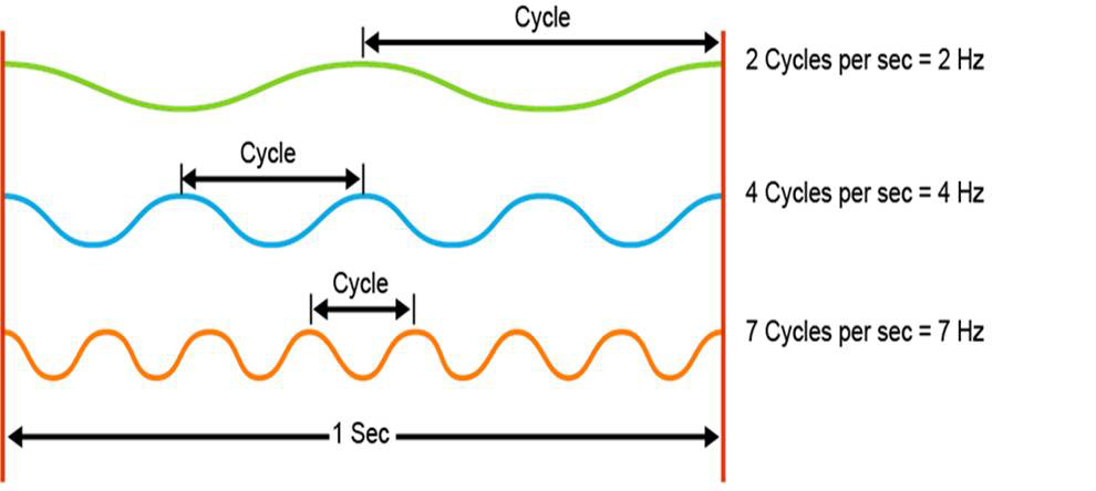
Figure 12-2 Cycles Within a Wave
A direct relationship exists between the frequency of a signal (how often the signal is seen) and the wavelength of the signal (the distance that the signal travels in one cycle). The shorter the wavelength, the more often the signal repeats over a given amount of time and, therefore, the higher the frequency.
A signal that occurs 1 million times per second is a megahertz, and a signal that occurs 1 billion times per second is a gigahertz. This fact is important in Wi-Fi networks because lower-frequency signals are less affected by the air than are high-frequency signals.
Wavelength
An RF signal starts with an electrical alternating current (AC) signal that a transmitter generates. This signal is sent through a cable to an antenna, which radiates the signal in the form of an electromagnetic wireless signal. Changes of electron flow in the antenna, known as current, produce changes in the electromagnetic fields around the antenna and transmit electric and magnetic fields.
AC is electrical current in which the direction of the current changes cyclically. The shape and form of an AC signal—the waveform—is known as a sine wave. This shape is the same as the signal that the antenna radiates on a wireless access point.
The physical distance from one point of a wave’s cycle to the same point in the next cycle is called a wavelength and is typically represented by the Greek symbol lambda (λ). The wavelength is the physical distance that the wave covers in one cycle. This is illustrated in Figure 12-3, where the waves are arranged in order of increasing frequency, from top to bottom. Notice that the wavelength decreases as the frequency increases.

Figure 12-3 Wireless Signal Transmission, with Examples of Increasing Frequency and Decreasing Wavelength
Wavelength distance determines some important properties of the wave. Certain environments and obstacles can affect the wave, and the degree of impact varies depending on the wavelength and the obstacle that the wave encounters. This phenomenon is covered in more detail later today.
Some AM radio stations use a wavelength that is 1312 or 1640 feet (400 or 500 m) long. Wi-Fi networks use a wavelength that is a few centimeters long. Some satellites use wavelengths that are about 0.04 inch (1 mm) long.
Amplitude
Amplitude is another important factor that affects how a wave is sent. Amplitude is the strength of a signal. In a graphical representation, amplitude is the distance between the highest and lowest crests of the cycle, as illustrated in Figure 12-4.

Figure 12-4 Signal Amplitude
The Greek symbol gamma (γ) is commonly used to represent amplitude. Amplitude affects the signal because it represents the level of energy that is injected in one cycle. The more energy that is injected in a cycle, the higher the amplitude.
Amplification is the increase of the amplitude of a wave. Amplification can be active or passive. In active amplification, the applied power is increased. Passive amplification is accomplished by focusing the energy in one direction by using an antenna. Amplitude can also be decreased. A decrease in amplitude is called attenuation.
Finding the right amplitude for a signal can be difficult. A signal weakens as it moves away from the emitter. If a signal is too weak, it might be unreadable when it arrives at the receiver. If a signal is too strong, then generating it requires too much energy (making the signal costly to generate). In addition, high signal strength can damage a receiver.
Regulations exist for determining the right amount of power to use for each type of device, depending on the expected distance over which the signal will be sent. Following these regulations helps avoid problems related to using the wrong amplitude.
Free Path Loss
A radio wave that an access point (AP) emits is radiated in the air. With an omnidirectional antenna, the signal is emitted in all directions—as when a stone is thrown into water, and waves radiate outward from the point at which the stone touches the water. If an AP uses a directional antenna, the beam is more focused in one direction.
As the signal or wave travels away from the AP, it is affected by any obstacles that it encounters. The exact effect depends on the type of obstacle the wave encounters. Even without encountering any obstacle, the first effect of wave propagation is strength attenuation.
Continuing with the example of a stone being thrown into water, the generated radio wave circles have higher crests close to the center than they do farther out. As the distance increases, the circles become flatter, until they finally disappear completely.
The attenuation of signal strength on its way between a sender and a receiver is called free path loss, or free space path loss. The word free in this case refers to the fact that the loss of energy is simply a result of distance; that is, it is not due to any obstacle. Path loss, on the other hand, also considers other sources of loss.
Keep in mind that what causes free path loss is not distance itself; there is no physical reason for a signal to be weaker farther away from the source. The cause of the loss is actually the combination of two phenomena:
• The signal is sent from the emitter in all directions. The energy must be distributed over a larger area (a larger circle), but the amount of energy that is originally sent does not change. Therefore, the amount of energy that is available on each point of the circle is higher if the circle is small (with fewer points) than if the circle is large (with more points among which the energy must be divided).
• The receiver antenna has a certain physical size, and the amount of energy that is collected depends on this size. A large antenna collects more points of the circle than a small one. But regardless of size, an antenna cannot pick up more than a portion of the original signal, especially because this process occurs in three dimensions (whereas the stone in water example occurs in two dimensions); the rest of the sent energy is lost.
The combination of these two factors causes free path loss. If energy could be emitted toward a single direction and if the receiver could catch 100% of the sent signal, there would be no loss at any distance because there would be nothing along the path to absorb any signal strength.
Some antennas are built to focus the signal as much as possible to try to send a powerful signal far from the AP. But the focus is still not perfect, so receivers cannot capture 100% of what is sent.
RSSI and SNR
Because an RF wave can be affected by obstacles in its path, it is important to determine how much signal the other endpoint will receive. The signal can become too weak for the receiver to hear or detect it as a signal. Two values are important in this determination: RSSI and SNR.
RSSI
Received signal strength indicator (RSSI), also called the signal value, indicates how much power is received. RSSI is the strength of a signal that one device receives from another device. RSSI is usually expressed in decibels referenced to 1 milliwatt (dBm).
Calculating RSSI is a complex problem because the receiver does not know how much power was originally sent. RSSI expresses a relative value that the receiving wireless network card determines while comparing received packets to each other.
RSSI is a grade value that can range from 0 (no signal or no reference) to a maximum of 255. However, many vendors use a maximum value that is lower than 255 (for example, 100 or 60). The value is relative because a magnetic field and an electric field are received, and a transistor transforms them into electric power; current is not directly received. How much electric power can be generated depends on the received field and the circuit that transforms it into current.
From the RSSI grade value, an equivalent dBm value is displayed, and this value depends on the vendor. One vendor might determine that the RSSI for a card will range from 0 to 100, where 0 is represented as –95 dBm and 100 as –15 dBm; another vendor might determine that the range will be 0 to 60, where 0 is represented as –92 dBm and 60 as –12 dBm. In this case, it is not possible to compare powers when reading RSSI = –35 dBm on the first product and RSSI = –28 dBm on the second product. For Cisco products, good RSSI values would be –67 dBm or better (for example, –55 dBm).
Therefore, RSSI is not a means of comparing wireless network cards; rather, it is a way to help understand, card by card, how strong a received signal is relative to itself in different locations. This method is useful for troubleshooting or when comparing the values of cards by the same vendor.
An attempt is being made to unify these values through the received channel power indicator (RCPI). Future cards might use the RCPI, which will be the same scale on all cards, instead of RSSI.
Noise (or noise floor) can be caused by wireless devices, such as cordless phones and microwaves. The noise value is measured in decibels, from 0 to –120. The noise level is the amount of interference in the Wi-Fi signal, and the lower value, the better. A typical noise floor value would be –95 dBm.
SNR
Another important metric is signal-to-noise ratio (SNR). SNR is a ratio value that evaluates a signal, based on the noise present. SNR is measured as a positive value between 0 and 120; the closer the value is to 120, the better.
SNR comprises two values, as shown in Figure 12-5:
• RSSI
• Noise (any signal that interferes with the signal)
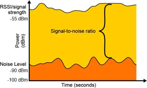
Figure 12-5 SNR Example
To calculate the SNR value, subtract the noise value from the RSSI. Because both values are usually expressed as negative numbers, the result is a positive number that is expressed in decibels. For example, if the RSSI is –55 dBm and the noise value is –90 dBm, you can make the following calculation:
–55 dBm – (–90 dBm) = –55 dBm + 90 dBm = 45 dBm
So in this case, you have an SNR of 45 dB. The general principle is that any SNR above 20 dB is good. These values depend not only on the background noise but also on the speed that is to be achieved.
As an example of SNR in everyday life, when someone speaks in a room, a certain volume is enough to be heard and understood. But if the same person speaks outdoors, surrounded by the noise of traffic, the same volume might be enough to be heard but not enough to be understood. In a very quiet room, a whisper can be heard. Although the voice is almost inaudible, it is easy to understand because it is the only sound present. In a noisy outdoor environment, isolating the voice from the surrounding noise is more difficult, and the voice needs to be much louder than the surrounding noise to be understood.
Current calculations use the signal-to-interference-plus-noise ratio (SINR). This calculation takes into account the noise floor and the strength of any interference to the signal. An SINR calculation is the RSSI minus the combination of interference and noise. An SINR of 25 or better is required for voice over wireless LAN (VoWLAN) applications.
Watts and Decibels
A key problem in Wi-Fi network design is determining how much power is or should be sent from a source and, therefore, is or should be received by the endpoint. The distances that can be achieved depend on this determination. The power that is sent from a source also determines which device to install, the type of AP to use, and the type of antenna to use.
The first unit of power that is used in power measurement is the watt (W), which is named after James Watt. The watt is a measure of the energy spent (that is, emitted or consumed) per second; 1 W represents 1 joule (J) of energy per second. A joule is the amount of energy that is generated by a force of 1 newton (N) moving 1 meter in one direction. A newton is the force that is required to accelerate 1 kg at a rate of 1 meter per second squared (m/s2).
Watt or milliwatt is an absolute power value that simply expresses power consumption. These measurements are also useful in comparing devices. For example, a typical AP can have a power of 100 mW, but this power varies depending on the context (indoor or outdoor) and the country because there are some regulations in this field.
Another value that is commonly used in Wi-Fi networks is the decibel (dB), which is used to indicate sound levels. A decibel is a logarithmic unit of measurement that expresses the amount of power relative to a reference.
Calculating decibels can be more challenging than simply understanding them. To simplify the task, remember these main values:
• 10 dB: When the power is 10 dB, the compared value is 10 times more powerful than the reference value. This process also works around the other way: If the compared value is 10 times less powerful than the reference value, then the compared value is written as –10 dB.
• 3 dB: Remember that decibels are logarithmic. If the power is 3 dB, then the compared value is twice as powerful as the reference value. By the same logic, if the compared value is half as powerful as the reference value, then the compared value is written as –3 dB.
Decibels are used extensively in Wi-Fi networks to compare powers. Two types of powers can be compared:
• The electric power of a transmitter
• The electromagnetic power of an antenna
Since the signal that a transmitter emits is an AC current, the power levels are expressed in milliwatts. Comparing powers between transmitters involves comparing values in milliwatts and using dBm as the units.
Following the rules regarding decibels and keeping in mind that a decibel expresses a relative value, you can establish these facts:
• A device that sends at 0 dBm sends the same number of milliwatts as the reference source. If the power reference is 1 mW, the device sends 1 mW.
• A device that sends at 10 dBm sends 10 times as much power (in milliwatts) than the reference source. If the power reference is1 mW, the device sends 10 mW.
• A device that sends at –10 dBm is one-tenth as powerful as the reference source. If the power reference is 1 mW, the device sends 0.1 mW.
• A device that sends at 3 dBm is twice as powerful as the reference source and sends 2 mW.
• A device that sends at –3 dBm is half as powerful as the reference source and sends 0.5 mW.
These calculations are illustrated in Figure 12-6.

Figure 12-6 Watts to Decibels
By the same logic, a device that sends 6 dBm is four times as powerful as the reference source: Adding 3 dBm makes the device twice as powerful and adding another 3 dBm, which makes it twice as powerful again, for a total of 4 mW.
The rules of 3 and 10 allow you to easily determine the transmit power, based on the gain or loss of decibels:
• +3 dB = power times 2
• –3 dB = power divided by 2
• +10 dB = power times 10
• –10 dB = power divided by 10
So, for every gain of 3 dB, the power is multiplied by 2, and for every gain of 10 dB, the power is multiplied by 10. Conversely, for –3 dB, the power is divided by 2, and for –10 dB, the power is divided by 10. These rules can help you more easily perform calculations of power levels.
Antenna Power
An antenna does not send an electric current; rather, an antenna sends an electromagnetic field. Wi-Fi engineers need to compare the power of antennas without using the indirect value of the current that is sent, and they do so by measuring the power gain relative to a reference antenna.
This reference antenna, called an isotropic antenna, is a spherical antenna that is theoretically 1 dot large and radiates in all directions, as shown in Figure 12-7. This type of antenna is theoretical and does not exist in reality for two reasons:
• An antenna that is 1 dot large is almost impossible to produce because something would need to be linked to the antenna to send the current to it.
• An antenna usually does not radiate equally in all directions because its construction causes it to send more signal in some directions than in others.
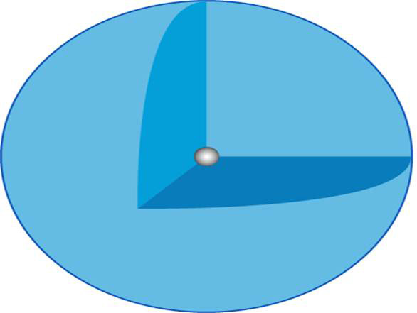
Figure 12-7 Theoretical Isotropic Antenna
Although this theoretical antenna does not exist, it can be used as a reference to compare actual antennas. The scale that is used to compare the powers that antennas radiate to an isotropic antenna is called dBi (where the i stands for isotropic).
The logarithmic progression of the dBi scale obeys the same rules as for the other decibel scales:
• 3 dBi is twice as powerful as the theoretical reference antenna.
• 10 dBi is 10 times as powerful as the theoretical reference antenna.
By using the same logarithmic progression, you can compare antennas similarly to the way you compare transmitters. For example, if one antenna is 6 dBi and another is 9 dBi, then the second antenna is 3 dBi more powerful than the first—or two times as powerful.
Other scales can be used to compare antennas. Some Wi-Fi professionals prefer to use a dipole antenna as the reference. This comparison is expressed in dBd. When comparing antennas, be sure to use the same format (either dBd or dBi) for all the antennas involved in the comparison.
Effective Isotropic-Radiated Power
Comparing antennas gives a measure of their gain. An antenna is a passive device, which means it does not add to the energy that it receives from the cable. The only thing that the antenna can do is to radiate the power in one or more directions.
An easy way to understand this concept is to consider a balloon as an example. The quantity of air inside the balloon is the quantity of energy to be radiated. If the balloon is shaped as a sphere, with an imaginary AP at the center, the energy is equally distributed in all directions. The imaginary AP at the center of the balloon radiates in all directions, like an isotropic antenna. Now suppose that the balloon is pressed into the shape of a sausage, and the imaginary AP is placed at one end of this sausage. The quantity of air in the balloon is still the same, but now the energy radiates more in one direction (along the sausage) than in the others.
The same principle applies to antennas. When an antenna concentrates the energy that it receives from the cable in one direction, it is said to be more powerful (in this direction) than an antenna that radiates the energy in all directions because there is more signal in this one direction.
In this sense, describing the power of antennas is like comparing their ability to concentrate the flow of energy in one direction. The more powerful an antenna, the higher its dBi or dBd value, the more it focuses or concentrates the energy that it receives into a narrower beam. But the total amount of power that is radiated is no higher; the antenna does not actively add power to what it receives from the transmitter.
Nevertheless, in the direction toward which the beam is concentrated, the received energy is higher because the receiver gets a higher percentage of the energy that the transmitter emits. And if the transmitter emits more energy, the result is higher yet.
Wi-Fi engineers need a way to determine how much energy is actually radiated from an antenna toward the main beam. This measure is called effective isotropic-radiated power (EIRP). One important concept to keep in mind is that EIRP is isotropic because it is the amount of power that an isotropic antenna would need to emit to produce the peak power density observed in the direction of maximum antenna gain. In other words, EIRP expresses, in isotropic equivalents, how much energy is radiated in the beam. Of course, to do so, EIRP takes into consideration the beam shape and strength and the antenna specifications.
In mathematical terms, EIRP, expressed in dBm, is simply the amount of transmit (Tx) power plus the gain (in dBi) of the antenna. However, the signal might go through a cable, and some power might be lost in the cable, so the cable loss must be deducted.
Therefore, EIRP can be expressed as EIRP = Tx power (dBm) + Antenna gain (dBi) – Cable loss (dB), as shown in Figure 12-8.

Figure 12-8 EIRP Calculation Example
EIRP is important from a resulting power and regulations standpoint. Most countries allow a maximum Tx power of the transmitter and a final maximum EIRP value, which is the resulting power when the antenna is added. An installer must pick the appropriate antenna and transmitter power settings, based on regulations for the country of deployment.
For example, say that you want to calculate the EIRP for a deployment with the following parameters:
• Tx power = 10 dBm
• Antenna gain = 6 dBi
• Cable loss = –3 dB
The EIRP in this case is calculated as 10 + 6 – 3 = 13 dBm.
IEEE Wireless Standards
This section discusses the IEEE 802.11 wireless communication standards for channels, data rates, and transmission techniques in Wi-Fi devices.
802.11 Standards for Channels and Data Rates
Being able to use a band, or range, of frequencies does not mean you can use it in any way you like. Important elements, such as which modulation technique to use, how a frame should be coded, which type of headers should be in the frame, and what the physical transmission mechanism should be, must be defined in order for devices to communicate with one another effectively.
The IEEE 802.11 standard defines how Wi-Fi devices should transmit in the Industrial, Scientific, and Medical (ISM) band. Today, whenever a Wi-Fi device is used, its Layer 1 and Layer 2 functionalities—such as receiver sensitivity, MAC layer performance, data rates, and security—are defined by an IEEE 802.11 series protocol.
802.11b/g
The 802.11b standard, which was ratified in 1999, offers rates of 5.5 to 11 Mbps and operates in the 2.4 GHz spectrum.
The IEEE 802.11g standard, which was ratified in June 2003, operates in the same spectrum as 802.11b and is backward compatible with the 802.11b standard. 802.11g supports additional data rates of 6, 9, 12, 18, 24, 36, 48, and 54 Mbps. 802.11g delivers the same 54 Mbps maximum data rate as 802.11a but operates in the same 2.4 GHz band as 802.11b.
802.11b and 802.11g once had broad user acceptance and vendor support, but due to their use of the 2.4 GHz band, which is prone to interference from other devices, and the slower speeds than are available with the newer 802.11 standards, the 802.11b/g standards are rarely used in today’s enterprise networks.
802.11a
The IEEE ratified the 802.11a standard in 1999. 802.11a, which delivers a maximum data rate of 54 Mbps, uses orthogonal frequency-division multiplexing (OFDM), which is a multicarrier system (as opposed to a single-carrier system). OFDM allows subchannels to overlap, so it provides high spectral efficiency, and the modulation technique that is allowed in OFDM is more efficient than the spread-spectrum techniques used with 802.11b. Operating in an unlicensed portion of the 5 GHz radio band, 802.11a is also immune to interference from devices that operate in the 2.4 GHz band.
Since this band is different from the 2.4 GHz-based products, 802.11a chips were initially expensive to produce. With 802.11g providing the same speed at 2.4 GHz and at longer distances, 802.11a has never had broad user acceptance. The slower speeds available with 802.11a than with the newer 802.11 standards has led to the 802.11a standard rarely being used in today’s enterprise network.
802.11n
802.11n, which was ratified in September 2009, is backward compatible with 802.11a and 802.11b/g and provides throughput enhancements. Features include channel bonding for up to 40 MHz channels, packet aggregation, and block acknowledgment. In addition, improved signals thanks to multiple-input, multiple-output (MIMO) enable clients to connect with faster data rates at a given distance from the AP compared to 802.11a/b/g. The 802.11n MIMO antenna technology extends data rates into the hundreds of megabits per second in the 2.4 and 5 GHz bands, depending on the number of transmitters and receivers that the devices implement.
802.11ac
IEEE 802.11ac was ratified in December 2013. Like 802.11a, it operates in the 5 GHz spectrum. The initial deployment, “Wave 1,” uses channel bonding for up to 80 MHz channels, 256-QAM coding, and one to three spatial streams, providing data rates up to 1.27 Gbps. “Wave 2” uses up to 160 MHz channel bonding, one to eight spatial streams, and multi-user MIMO (MU-MIMO), providing data rates up to 6.77 Gbps.
An 802.11ac device supports all mandatory modes of 802.11a and 802.11n. So, an 802.11ac AP can communicate with 802.11a and 802.11n clients using 802.11a- or 802.11n-formatted packets, and it is as if the AP were an 802.11n AP. Similarly, an 802.11ac client can communicate with an 802.11a or 802.11n AP by using 802.11a or 802.11n packets. Therefore, 802.11ac clients do not cause issues with an existing infrastructure.
802.11ax (Wi-Fi 6)
IEEE 802.11ax is a standards draft that is expected to be ratified in late 2020. The Wi-Fi Alliance has branded the standard Wi-Fi 6. The first wave of IEEE 802.11ax access points support eight spatial streams and 80 MHz channels, deliver up to 4.8 Gbps at the physical layer. Unlike 802.11ac, 802.11ax is a dual-band 2.4 and 5 GHz technology, so legacy 2.4 GHz–only clients can take advantage of its benefits. Wi-Fi 6 will also support 160 MHz–wide channels and will be able to achieve the same 4.8 Gbps speeds with fewer spatial streams.
Like 802.11ac, the 802.11ax standard also supports downlink MU-MIMO, which means a device can transmit to multiple receivers concurrently. However, 802.11ax also supports uplink MU-MIMO, which means a device can simultaneously receive from multiple transmitters.
802.11n/802.11ac MIMO
Today, APs and clients that support only the 802.11a/b/g protocols are considered legacy systems. Such a system uses a single transmitter that talks to a single receiver to provide a connection to the network. A legacy device that uses single-input, single-output (SISO) has only one radio that switches between antennas. When receiving a signal, the radio determines which antenna provides the strongest signal and switches to the best antenna. However, only one antenna is used at a time. This is illustrated at the top of Figure 12-9.

Figure 12-9 802.11n and 802.11ac MIMO
This configuration leaves both the AP and the client susceptible to degraded performance when confronted by reflected copies of the signal—a phenomenon that is known as multipath reception.
802.11n/ac makes use of multiple antennas and radios, which are combined with advanced signal-processing methods to implement a technique known as multiple-input, multiple-output (MIMO). Several transmitter antennas send several frames over several paths. Several receiver antennas recombine these frames to optimize throughput and multipath resistance.
MIMO effectively improves the reliability of a Wi-Fi link, provides better SNR, and therefore reduces the likelihood that packets will be dropped or lost.
When MIMO is deployed only in APs, the technology delivers significant performance enhancements (as much as 30% over conventional 802.11a/b/g networks) even when communicating only with non-MIMO 802.11a/b/g clients by using a feature called Cisco ClientLink.
For example, at the distance from the AP at which an 802.11a or 802.11g client communicating with a conventional AP might drop from 54 to 24 Mbps, the same client communicating with a MIMO-enabled AP might be able to continue operating at 54 Mbps. This is illustrated in the middle of Figure 12-9.
Ultimately, 802.11 networks that incorporate both MIMO-enabled APs and MIMO-enabled Wi-Fi clients deliver dramatic gains in reliability and data throughput, as illustrated at the bottom of Figure 12-9.
MIMO incorporates three main technologies:
• Maximum-ratio combining (MRC)
• Beamforming
• Spatial multiplexing
Maximal Ratio Combining
A receiver with multiple antennas uses maximum-ratio combining (MRC) to optimally combine energies from multiple receive chains. An algorithm eliminates out-of-phase signal degradation.
Spatial multiplexing and Tx beamforming are used when there are multiple transmitters. MRC is the counterpart of Tx beamforming and takes place on the receiver side—usually on the AP—regardless of whether the client sender is 802.11n compatible. The receiver must have multiple antennas to use this feature, and 802.11n APs usually do. The MRC algorithm determines how to optimally combine the energy that is received at each antenna so that each signal that transmits to the AP circuit adds to the others in a coordinated fashion. In other words, the receiver analyzes the signals it receives from all its antennas and sends the signals into the transcoder so that they are in phase, thereby adding the strength of each signal to the other signals. At the top of Figure 12-10, only one weak signal is received by the AP. At the bottom of the figure, the AP receives three signals from the station. MRC combines these individual signals, allowing for faster data rates to be maintained between AP and client.
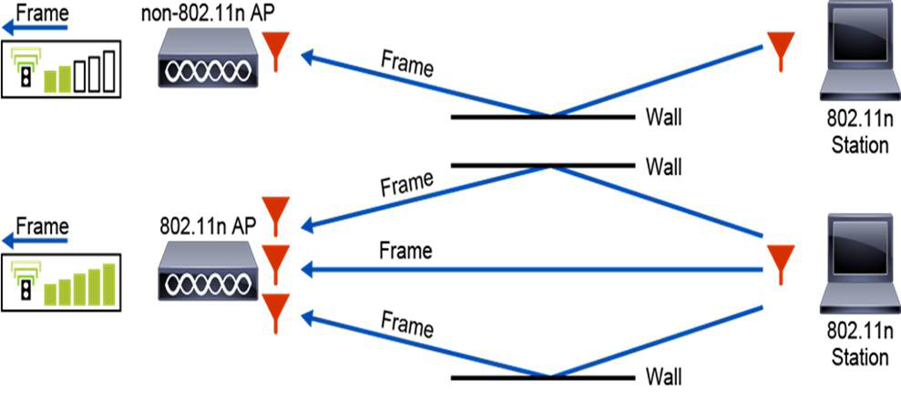
Figure 12-10 Maximum-Ratio Combining
Note that MRC is not related to multipath. Multipath issues are due to one antenna receiving reflected signals out of phase. This out-of-phase result, which is destructive to the signal quality, is transmitted to the AP. MRC combines the signals that come from two or three physically distinct antennas in a timely fashion so that the signals that are received on the antennas are in phase. The system evaluates the state of the channel for the signal that is received on each antenna and chooses the best received signal for each symbol, thereby ignoring pieces of waves on one chain that would not be read well. This system increases the quality of the reception. If you have, for example, three receive chains, you have three chances to read each symbol that is received, so MRC can minimize the possibility of interference degrading the section of the wave on all three receivers.
Multipath might still play a role. For example, each antenna might receive a reflected signal out of phase, and the antenna will be able to transmit to the AP only what it receives. The main advantage of MRC in this case is that, because each antenna is physically separated from the others, the received signals on each antenna are affected differently by multipath issues. When all the signals are added together, the result will be closer to the wave that was sent by the sender, and the relative impact of multipath on each antenna will be less predominant.
Beamforming
Tx beamforming is a technique that is used when there is more than one Tx antenna. The signals sent from the antennas can be coordinated so that the signal at the receiver is dramatically improved, even if the antenna is far from the sender.
This technique is generally used when the receiver has only one antenna and when the reflection sources are stable in space (such as with a receiver that is not moving fast and an indoor environment), as illustrated in Figure 12-11.
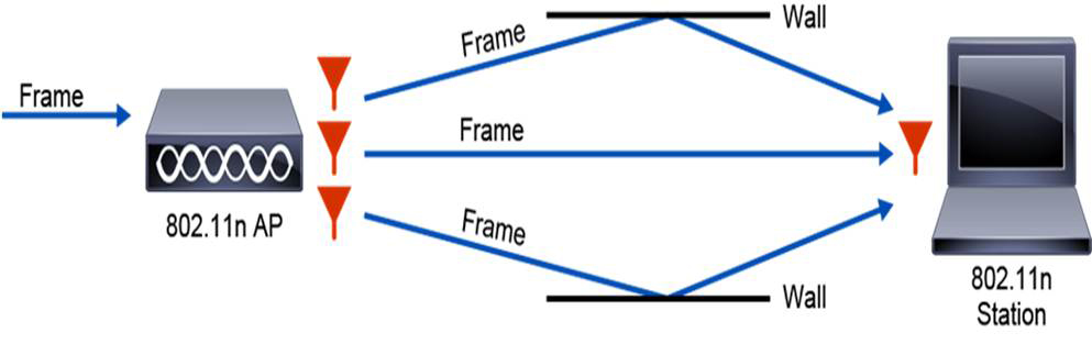
Figure 12-11 Beamforming
An 802.11n-capable transmitter may perform Tx beamforming. This technique allows the 802.11n-capable transmitter to adjust the phase of the signal that is transmitted on each antenna so that the reflected signals arrive in phase with one another at the receive (Rx) antenna. This technique can be applied even on a legacy client that has a single Rx antenna. Having multiple signals arrive in phase with one another effectively increases the Rx sensitivity of the single radio of a legacy client. This technique is software-defined beamforming.
802.11n added the opportunity for the receiver to help the beamforming transmitter do a better job of beamforming. This process, called sounding, enables the beamformer to precisely steer its transmitted energy toward the receiver. 802.11ac defines a single protocol for one 802.11ac device to sound other 802.11ac devices. The protocol that is selected loosely follows the 802.11n explicit compressed feedback protocol.
Explicit beamforming requires that the AP and the client have the same capabilities. The AP dynamically gathers information from the client in order to determine the best path. Implicit beamforming uses some information from the client at the initial association. Implicit beamforming improves the signal for older devices.
802.11n originally specified how MIMO technology can be used to improve SNR at the receiver by using Tx beamforming. However, both the AP and the client need to support this capability.
Cisco ClientLink technology helps solve the problems of mixed-client networks by making sure that older 802.11a/n clients operate at the best possible rates, especially when they are near cell boundaries. ClientLink also supports the ever-growing number of 802.11ac clients that support one, two, or three spatial streams. Unlike most 802.11ac APs, which improve only uplink performance, Cisco ClientLink improves performance on both the uplink and the downlink, providing better user experiences with web browsing, email, and file downloads. ClientLink technology is based on signal-processing enhancements to the AP chipset and does not require changes to network parameters.
Spatial Multiplexing
Spatial multiplexing requires both an 802.11n/ac-capable transmitter and an 802.11n/ac-capable receiver. It requires a minimum of two receivers and a single transmitter per band and supports as many as four transmitters and four receivers per band. Spatial multiplexing allows the advanced signaling processes of 802.11n to effectively use the reflected signals that are detrimental to legacy protocols. The reflected signals allow this technology to function. The reduction in lost packets improves link reliability, which results in fewer retransmissions. Ultimately, the result is more consistent throughput, which helps ensure predictable coverage throughout a facility.
With spatial multiplexing, a signal stream is broken into multiple individual streams, each transmitted from a different antenna, using its own transmitter. Because there is space between antennas, each signal follows a different path to the receiver. This phenomenon, known as spatial diversity, is illustrated in Figure 12-12. Each radio can send a different data stream from the other radios, and all radios can send at the same time, using a complex algorithm that is built on feedback from the receiver.
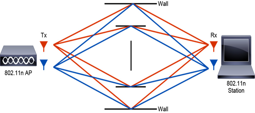
Figure 12-12 Spatial Multiplexing
The receiver has multiple antennas, each with its own radio. Each receiver radio independently decodes the arriving signals. Then each Rx signal is combined with the signals from the other radios. Thanks to a lot of complex math, the result is a much better Rx signal that can be achieved with either a single antenna or with Tx beamforming. Using multiple streams allows 802.11n devices to send redundant information for greater reliability, a greater volume of information for improved throughput, or a combination of the two.
For example, consider a sender that has two antennas. The data is broken into two streams that two transmitters transmit at the same frequency. The receiver says, "Using my three Rx antennas with my multipath and math skills, I can recognize the two streams that are transmitted at the same frequency because the transmitters have spatial separation."
A Wi-Fi network is more efficient when it uses MIMO spatial multiplexing, but there can be a difference between the sender and the receiver. When a transmitter can emit over three antennas, it is described as having three data streams. When it can receive and combine signals from three antennas, it is described as having three receive chains. The combination of three data streams and three receive chains is commonly denoted as three by three (3X3). Similarly, there are 2X2, 4X4, and 8X8 devices, which have two, four, and eight spatial streams, respectively.
An 802.11ac environment allows more data by increasing the spatial streams to up to eight. Therefore, an 80 MHz channel with one stream provides a throughput of 300 Mbps, while eight streams provide a throughput of 2400 Mbps. Using a 160 MHz channel would allow throughput of 867 Mbps (one stream) to 6900 Mbps (eight streams).
802.11ac MU-MIMO
With 802.11n, a device can transmit multiple spatial streams at once—but only directed to a single address. For individually addressed frames, this means that only a single device (or user) receives data at a time. This is called single-user MIMO (SU-MIMO). 802.11ac provides for a feature called multi-user MIMO (MU-MIMO), in which an AP uses its antenna resources to transmit multiple frames to up to four different clients, all at the same time and over the same frequency spectrum, as illustrated in Figure 12-13.

Figure 12-13 MU-MIMO Using a Combination of Beamforming and Null Steering to Multiple Clients in Parallel
To send data to user 1, the AP forms a strong beam toward user 1 (shown as the top-right lobe of the color curve). At the same time, the AP minimizes the energy for user 1 in the direction of user 2 and user 3. This circumstance is called null steering and is shown as the color notches. In addition, the AP is sending data to user 2, forms a beam toward user 2, and forms notches toward users 1 and 3, as shown by the color curve. The color curve shows a similar beam toward user 3 and nulls toward users 1 and 2. In this way, each of users 1, 2, and 3 receives a strong copy of the desired data that is only slightly degraded by interference from data for the other users.
MU-MIMO allows an AP to deliver appreciably more data to its associated clients, especially for small form-factor clients (often BYOD clients) that are limited to a single antenna each. If the AP is transmitting to two or three clients, the effective speed increase varies from a factor of unity (no speed increase) up to a factor of two or three times, depending on the Wi-Fi channel conditions. If the speed-up factor drops below unity, the AP uses SU-MIMO instead.
Study Resources
For today’s exam topics, refer to the following resources for more study.
