Day 14. Network Assurance, Part 1
ENCOR 350-401 Exam Topics
• Network Assurance
• Diagnose network problems using tools such as debugs, conditional debugs, trace route, ping, SNMP, and syslog
• Configure and verify SPAN/RSPAN/ERSPAN
• Configure and verify IPSLA
Key Topics
Today we start our review of concepts related to network assurance. Network outages that cause business-critical applications to become inaccessible could potentially cause an organization to sustain significant financial losses. Network engineers are often asked to perform troubleshooting in these cases. Troubleshooting is the process of responding to a problem that leads to its diagnosis and resolution.
Today we first examine the diagnostic principles of troubleshooting and how they fit into the overall troubleshooting process. We also explore various Cisco IOS network tools used in the diagnostic phase to assist in monitoring and troubleshooting an internetwork. We also look at how to use network analysis tools such as Cisco IOS CLI troubleshooting commands, as well as Cisco IP service-level agreements (SLAs) and different implementations of switched port analyzer services, such as Switched Port Analyzer (SPAN), Remote SPAN (RSPAN), and Encapsulated Remote SPAN (ERSPAN).
On Day 13, “Network Assurance, Part 2,” we will discuss network logging services that can collect information and produce notifications of network events, such as syslog, Simple Network Management Protocol (SNMP), and Cisco NetFlow. These services are essential in maintaining network assurance and high availability of network services for users.
Troubleshooting Concepts
In general, the troubleshooting process starts when someone reports a problem. In a way, you could say that a problem does not exist until it is noticed, considered a problem, and reported. You need to differentiate between a problem, as experienced by a user, and the cause of that problem. So, the time that a problem was reported is not necessarily the same as the time at which the event that caused that problem occurred. However, a reporting user generally equates the problem with the symptoms, while the troubleshooter equates the problem with the root cause.
If the Internet connection flaps on a Saturday in a small company outside operating hours, is that a problem? Probably not, but it is very likely that it will turn into a problem on Monday morning if it is not fixed by then.
Although the distinction between symptoms and the cause may seem philosophical, it is good to be aware of the communication issues that can potentially arise.
A troubleshooting process starts with reporting and defining a problem, as illustrated in Figure 14-1. It is followed by the process of diagnosing the problem. During this process, information is gathered, the problem definition is refined, and possible causes for the problem are proposed. Eventually, this process should lead to a diagnosis of the root cause of the problem.
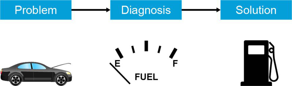
Figure 14-1 Basic Troubleshooting Steps
When the root cause has been found, possible solutions need to be proposed and evaluated. After the best solution is chosen, that solution should be implemented. Sometimes, the solution cannot be immediately implemented, and you need to propose a workaround until the solution can be implemented. The difference between a solution and a workaround is that a solution resolves the root cause of the problem, and a workaround only remedies or alleviates the symptoms of the problem.
Once the problem is fixed, all changes should be well documented. This information will be helpful the next time someone needs to resolve similar issues.
Diagnostic Principles
Although problem reporting and resolution are essential elements of the troubleshooting process, most troubleshooting time is spent in the diagnostic phase.
Diagnosis is the process in which you identify the nature and the cause of a problem. The essential elements of the diagnosis process are as follows:
• Gathered information: Gathering information about what is happening is essential to the troubleshooting process. Usually, the problem report does not contain enough information for you to formulate a good hypothesis without first gathering more information. You can gather information and symptoms either directly by observing processes or indirectly by executing tests.
• Analysis: The gathered information is analyzed. Compare the symptoms against your knowledge of the system, processes, and baseline to separate the normal behavior from the abnormal behavior.
• Elimination: By comparing the observed behavior against expected behavior, you can eliminate possible problem causes.
• Proposed hypotheses: After gathering and analyzing information and eliminating the possible causes, you are left with one or more potential problem causes. You need to assess the probability of each of these causes so that you can propose the most likely cause as the hypothetical cause of the problem.
• Testing: Test the hypothetical cause to confirm or deny that it is the actual cause. The simplest way to perform testing is to propose a solution that is based on this hypothesis, implement that solution, and verify whether it solves the problem. If this method is impossible or disruptive, the hypothesis can be strengthened or invalidated by gathering and analyzing more information.
Network Troubleshooting Procedures: Overview
A troubleshooting method is a guiding principle that determines how you move through the phases of the troubleshooting process, as illustrated in Figure 14-2.

Figure 14-2 Troubleshooting Process
In a typical troubleshooting process for a complex problem, you continually move between the different processes: Gather some information, analyze it, eliminate some possibilities, gather more information, analyze again, formulate a hypothesis, test it, reject it, eliminate some more possibilities, gather more information, and so on. However, the time spent on each of these phases and the method of moving from phase to phase can be significantly different from person to person and is a key differentiator between effective and less-effective troubleshooters.
If you do not use a structured approach but move between the phases randomly, you might eventually find the solution, but the process will be very inefficient. In addition, if your approach has no structure, it is practically impossible to hand it over to someone else without losing all the progress that was made up to that point. You also may need to stop and restart your own troubleshooting process.
A structured approach to troubleshooting (no matter what the exact method) yields more predictable results in the end and makes it easier to pick up the process where you left off in a later stage or to hand it over to someone else.
Network Diagnostic Tools
This section focuses on the use of the ping, traceroute, and debug IOS commands.
Using the ping Command
Using the ping command is a very common method for troubleshooting the accessibility of devices. ping uses a series of Internet Control Message Protocol (ICMP) echo request and echo reply messages to determine the following:
• Whether a remote host is active or inactive
• The round-trip delay in communicating with the host
• Packet loss
The ping command first sends an echo request packet to an address and waits for a reply. The ping is successful only if the following two conditions are true:
• The echo request gets to the destination.
• The destination can get an echo reply to the source within a predetermined time called a timeout. The default value of this timeout is 2 seconds on Cisco routers.
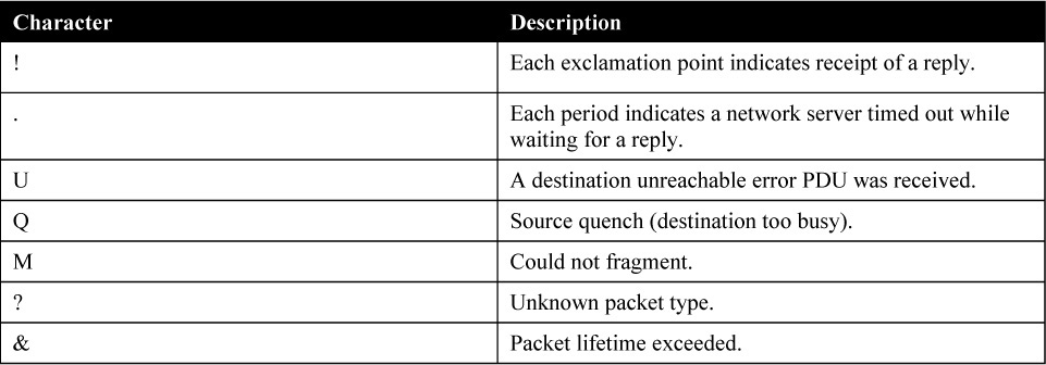
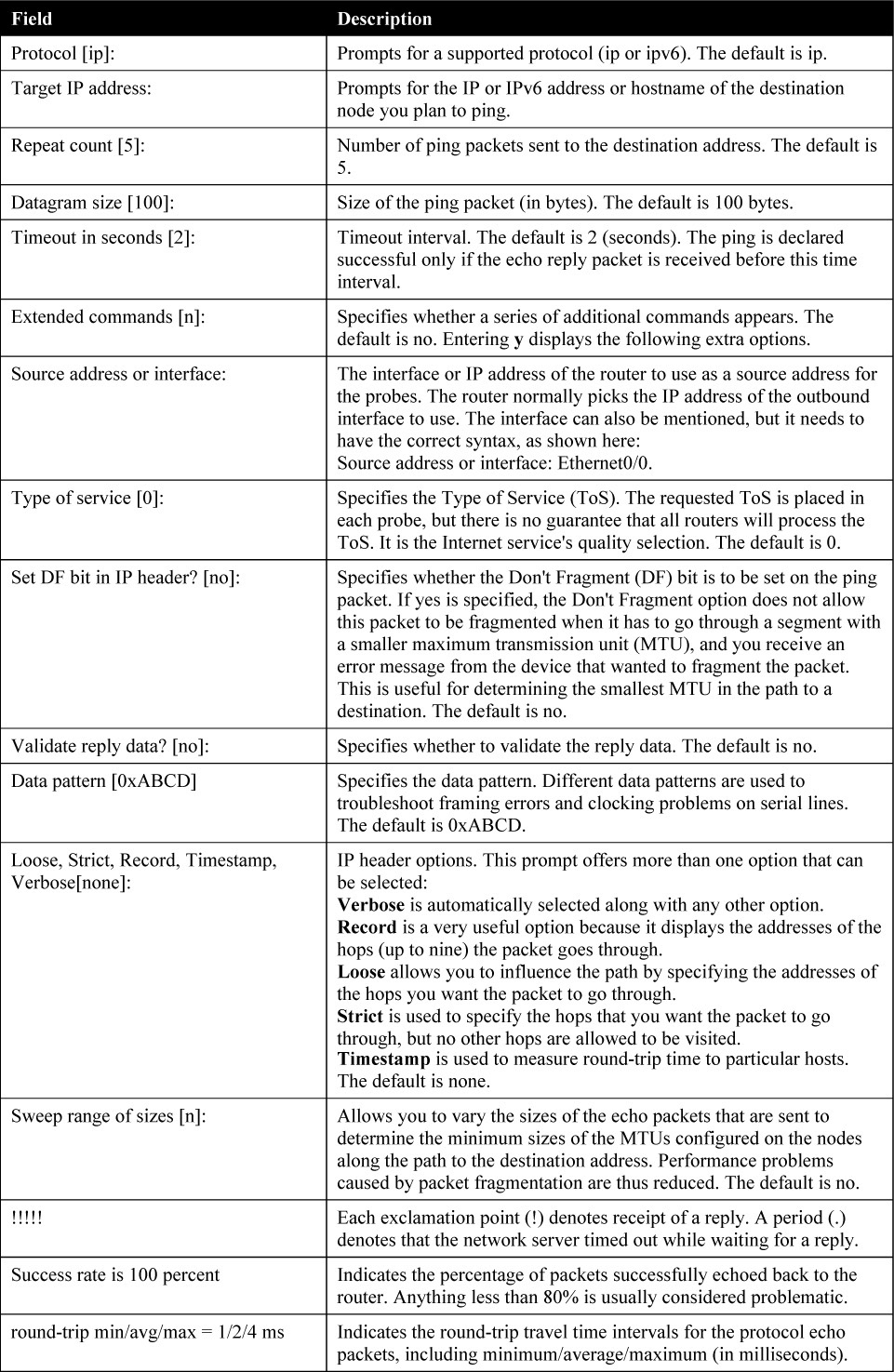
Table 14-1 lists the possible responses when conducting a ping test.
Table 14-1 Ping Characters
In Example 14-1, R1 has successfully tested its connectivity with a device at address 10.10.10.2.
Example 14-1 Testing Connectivity with ping
R1# ping 10.10.10.2

Type escape sequence to abort.
Sending 5, 100-byte ICMP Echos to 10.10.10.2, timeout is 2 seconds:
!!!!!
Success rate is 100 percent (5/5), round-trip min/avg/max = 1/201/1003 ms
R1#
When using the ping command, it is possible to specify options to help in the troubleshooting process. Example 14-2 shows some of these options.
Example 14-2 Ping Options
R1# ping 10.10.10.2 ?
  Extended-data  specify extended data pattern
  data           specify data pattern
  df-bit         enable do not fragment bit in IP header
  repeat         specify repeat count
  size           specify datagram size
  source         specify source address or name
  timeout        specify timeout interval
  tos            specify type of service value
  validate       validate reply data
  <cr>
The most useful options are repeat and source. The repeat keyword allows you to change the number of pings sent to the destination instead of using the default value of five. The source keyword allows you to change the interface used as the source of the ping. By default, the source interface is the router’s outgoing interface, based on the routing table. It is often desirable to test reachability from a different source interface instead.
The Extended Ping
The extended ping is used to perform a more advanced check of host reachability and network connectivity. To enter extended ping mode, type the ping keyword and immediately press Enter. Table 14-2 lists the options in an extended ping.
Table 14-2 Extended Ping Options
Example 14-3 shows R1 using the extended ping command to test connectivity with a device at address 10.10.50.2.
Example 14-3 Extended Ping Example
R1# ping
Protocol [ip]:
Target IP address: 10.10.50.2
Repeat count [5]: 1
Datagram size [100]:
Timeout in seconds [2]: 1
Extended commands [n]: y
Source address or interface:
Type of service [0]:
Set DF bit in IP header? [no]: y
Validate reply data? [no]:
Data pattern [0xABCD]:
Loose, Strict, Record, Timestamp, Verbose[none]:
Sweep range of sizes [n]: y
Sweep min size [36]: 1400
Sweep max size [18024]: 1500
Sweep interval [1]:
Type escape sequence to abort.
Sending 101, [1400..1500]-byte ICMP Echos to 10.10.50.2, timeout is 1 seconds:
Packet sent with the DF bit set
!!!!!!!!!!!!!!!!!!!!!!!!!!!!!!!!!!!!!!!!!!!!!!!!!!!!!!!!!!!!!!!!!!!!!!
!!!!!!!M.M.M.M.M.M.M.M.M.M.M.M.
Success rate is 76 percent (77/101), round-trip min/avg/max = 1/1/1 ms  <cr>
In this example, the extended ping is used to test the maximum MTU size supported across the network. The ping succeeds with a datagram size from 1400 to 1476 bytes and the Don’t Fragment-bit (df-bit) set; for the rest of the sweep, the result is that the packets cannot be fragmented. This outcome can be determined because the sweep started at 1400 bytes, 100 packets were sent, and there was a 76% success rate (1400 + 76 = 1476).
For testing, you can sweep packets at different sizes (minimum, maximum), set the sweeping interval, and determine the MTU by seeing which packets are passing through the links and which packets need to be fragmented since you have already set the df-bit for all the packets.
Using traceroute
The traceroute tool is very useful if you want to determine the specific path that a packet takes to its destination. If there is an unreachable destination, you can determine where on the path the issue lies.
The traceroute command works by sending the remote host a sequence of three UDP datagrams with a TTL of 1 in the IP header and the destination ports 33434 (first packet), 33435 (second packet), and 33436 (third packet). The TTL of 1 causes the datagram to time out when it hits the first router in the path. The router responds with an ICMP "time exceeded" message, indicating that the datagram has expired.
The next three UDP datagrams are sent with TTL of 2 to destination ports 33437, 33438, and 33439.
After passing through the first router, which decrements the TTL to 1, the datagram arrives at the ingress interface of the second router. The second router drops the TTL to 0 and responds with an ICMP "time exceeded" message. This process continues until the packet reaches the destination and the ICMP "time exceeded" messages have been sent by all the routers along the path.
Since these datagrams are trying to access an invalid port at the destination host, ICMP “port unreachable” messages are returned when the packet reaches the destination, indicating an unreachable port; this event signals that the traceroute program is finished.
The possible responses when conducting a traceroute are displayed in Table 14-3.
Table 14-3 traceroute Characters

Example 14-4 shows R1 performing a traceroute to a device at address 10.10.20.1.
Example 14-4 Testing Connectivity with traceroute
R1# traceroute 10.10.20.1
Type escape sequence to abort.
Tracing the route to 10.10.20.1
VRF info: (vrf in name/id, vrf out name/id)
  1 10.10.50.1 1 msec 0 msec 1 msec
  2 10.10.40.1 0 msec 0 msec 1 msec
  3 10.10.30.1 1 msec 0 msec 1 msec
  4 10.10.20.1 1 msec *  2 msec
R1#
In this example, R1 is able to reach the device at address 10.10.20.1 in four hops. The first three hops represent Layer 3 devices between R1 and the destination, and the last hop is the destination itself.
As with ping, it is possible to add optional keywords to the traceroute command to influence its default behavior, and it is also possible to perform an extended traceroute, which operates in a similar way to the extended ping command.
Using Debug
The output from debug commands provides diagnostic information that includes various internetworking events relating to protocol status and network activity in general.
Use debug commands with caution. In general, it is recommended that these commands be used only when troubleshooting specific problems. Enabling debugging can disrupt the operation of the router when internetworks are experiencing high load conditions. Hence, if logging is enabled, the device may intermittently freeze when the console port gets overloaded with log messages.
Before you start a debug command, always consider the output that the debug command will generate and the amount of time it can take. Before debugging, you might want to look at your CPU load with the show processes cpu command. Verify that you have ample CPU available before you begin the debugging.
Cisco devices can display debugging output on various interfaces or can be configured to capture the debugging messages in a log:
• Console: By default, logging is enabled on the console port. Hence, the console port always processes debugging output, even if you are actually using some other port or method (such as AUX, vty, or buffer) to capture the output. Excessive debugging to the console port of a router can cause it to hang. You should consider changing where the debugging messages are captured and turn off logging to the console with the no logging console command. Some debug commands are very verbose, and, therefore, you cannot easily view any subsequent commands you wish to type while these commands are in process. To remedy the situation, configure logging synchronous on the console line.
• AUX and vty ports: To receive debugging messages when connected to the AUX port or when remotely logged in to the device via Telnet or SSH through the vty lines, type the command terminal monitor.
• Logs: Like syslog messages, debugging messages can be collected in logs. You can use the logging command to configure messages to be captured in an internal device buffer or an external syslog server.
The debug ip packet command helps you better understand the IP packet forwarding process, but this command only produces information on packets that are process switched by the router.
Packets that are forwarded through a router that is configured for fast switching or CEF are not sent to the processor, and hence the debugging does not display anything about those packets. To display packets forwarded through a router with the debug ip packet command, you need to disable fast switching on the router with the no ip route-cache command for unicast packets or no ip mroute-cache for multicast packets. These command are configured on the interfaces where the traffic is supposed to flow. You can verify whether fast switching is enabled by using the show ip interface command.
The Conditional Debug
Another way of narrowing down the output of a debug command is to use a conditional debug command. If any debug condition commands are enabled, output is generated only for packets that contain information specified in the configured condition.
Table 14-4 lists the options available with a conditional debug command.
Table 14-4 Conditional Debug Options
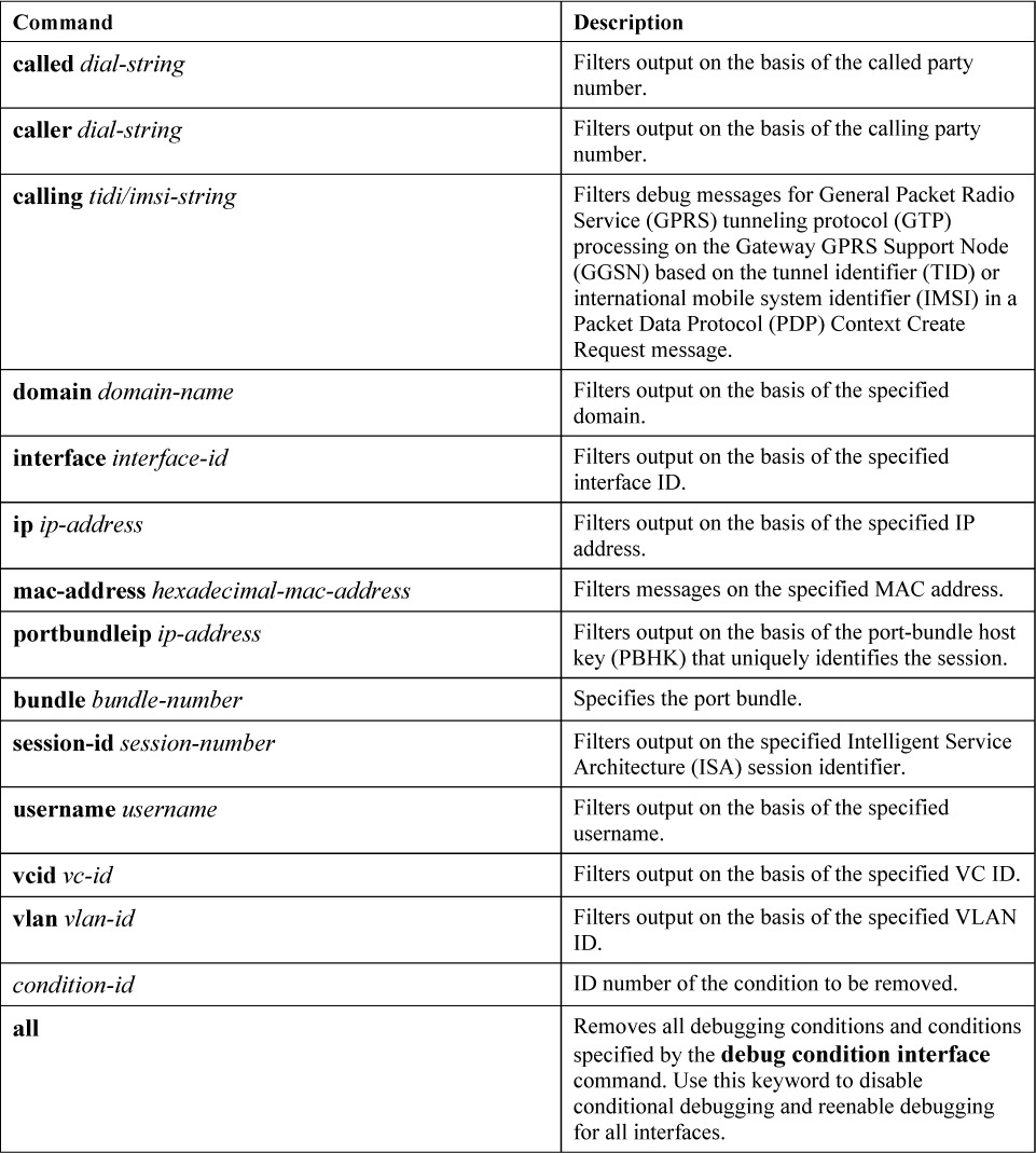
Example 14-5 shows the setting and verification of a debug condition for the GigabitEthernet 0/0/0 interface on R1. Any debug commands enabled on R1 would only produce logging output if there is a match on the GigabitEthernet 0/0/0 interface.
Example 14-5 Configuring and Verifying Conditional Debugs
R1# debug condition interface gigabitethernet 0/0/0
Condition 1 set
R1# show debug condition
Condition 1: interface Gi0/0/0 (1 flags triggered)
        Flags: Gi0/0/0
R1#
Another way of filtering debugging output is to combine the debug command with an access list. For example, with the debug ip packet command, you have the option to enter the name or number of an access list. Doing that causes the debug command to get focused only on packets that satisfy (that is, that are permitted by) the access list's statements.
In Figure 14-3, Host A uses Telnet to connect to Server B. You decide to use debug on the router connecting the segments where Host A and Server B reside.

Figure 14-3 Debugging with an Access List
Example 14-6 shows the commands used to test the Telnet session. Note that the no ip route-cache command was previously issued on R1’s interfaces.
Example 14-6 Using the debug Command with an Access List
R1(config)# access-list 100 permit tcp host 10.1.1.1 host 172.16.2.2 eq telnet
R1(config)# access-list 100 permit tcp host 172.16.2.2 eq telnet host 10.1.1.1 established
R1(config)# exit
R1# debug ip packet detail 100
IP packet debugging is on (detailed) for access list 100
HostA# telnet 172.16.2.2
Trying 172.16.2.2 ... Open

User Access Verification

Password:
ServerB>
R1
<. . . output omitted . . .>
*Jun  9 06:10:18.661: FIBipv4-packet-proc: route packet from Ethernet0/0 src 10.1.1.1 dst 172.16.2.2
*Jun  9 06:10:18.661: FIBfwd-proc: packet routed by adj to Ethernet0/1 172.16.2.2
*Jun  9 06:10:18.661: FIBipv4-packet-proc: packet routing succeeded
*Jun  9 06:10:18.661: IP: s=10.1.1.1 (Ethernet0/0), d=172.16.2.2 (Ethernet0/1), g=172.16.2.2, len 43, forward
*Jun  9 06:10:18.661:     TCP src=62313, dst=23, seq=469827330, ack=3611027304, win=4064 ACK PSH
*Jun  9 06:10:18.661: IP: s=10.1.1.1 (Ethernet0/0), d=172.16.2.2 (Ethernet0/1), len 43, sending full packet
*Jun  9 06:10:18.661:     TCP src=62313, dst=23, seq=469827330, ack=3611027304, win=4064 ACK PSH
*Jun  9 06:10:18.662: IP: s=172.16.2.2 (Ethernet0/1), d=10.1.1.1, len 40, input feature
*Jun  9 06:10:18.662:     TCP src=23, dst=62313, seq=3611027304, ack=469827321, win=4110 ACK, MCI Check(108), rtype 0, forus FALSE, sendself FALSE, mtu 0, fwdchk FALSE
<. . . output omitted . . .>
Considering the addressing scheme used in Figure 14-3, access list 100 permits TCP traffic from Host A (10.1.1.1) to Server B (172.16.2.2) with the Telnet port (23) as the destination. Access list 100 also permits established TCP traffic from Server B to Host A. Using access list 100 with the debug ip packet detail command allows you to see only debugging packets that satisfy the access list. This is an effective troubleshooting technique that requires less overhead on your router while allowing all information on the subject you are troubleshooting to be displayed by the debugging facility.
Cisco IOS IP SLAs
Network connectivity across the enterprise campus and also across the WAN and Internet from data centers to branch offices has become increasingly critical for customers, and any downtime or degradation can adversely affect revenue. Companies need some form of predictability with IP services. A service-level agreement (SLA) is a contract between a network provider and its customers or between a network department and its internal corporate customers. It provides a form of guarantee to customers about the level of user experience. An SLA typically outlines the minimum level of service and the expected level of service regarding network connectivity and performance for network users.
Typically, the technical components of an SLA contain a guaranteed level for network availability, network performance in terms of RTT, and network response in terms of latency, jitter, and packet loss. The specifics of an SLA vary depending on the applications that an organization is supporting in the network.
The tests generated by Cisco IOS devices used to determine whether an SLA is being met are called IP SLAs. IP SLA tests use various operations, as illustrated in Figure 14-4:
• FTP
• ICMP
• HTTP
• SIP
• Others
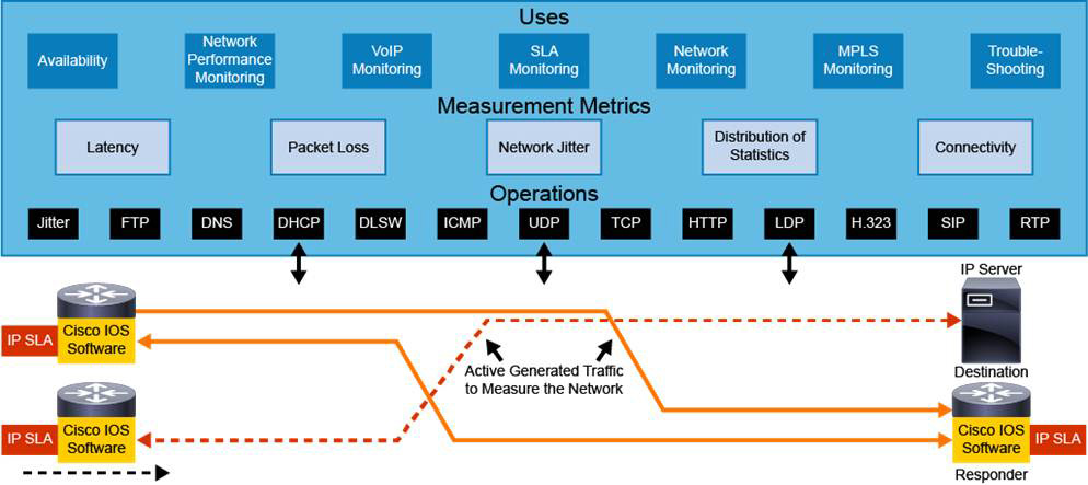
Figure 14-4 Cisco IOS IP SLA
These IP SLA operations are used to gather many types of measurement metrics:
• Network latency and response time
• Packet loss statistics
• Network jitter and voice quality scoring
• End-to-end network connectivity
These measurement metrics provide network administrators with the information for various uses, including the following:
• Edge-to-edge network availability monitoring
• Network performance monitoring and network performance visibility
• VoIP, video, and VPN monitoring
• SLA monitoring
• IP service network health
• MPLS network monitoring
• Troubleshooting of network operations
The networking department can use IP SLAs to verify that the service provider is meeting its own SLAs or to define service levels for its own critical business applications. An IP SLA can also be used as the basis for planning budgets and justifying network expenditures.
Administrators can ultimately reduce the mean time to repair (MTTR) by proactively isolating network issues. They can then change the network configuration, which is based on optimized performance metrics.
IP SLA Source and Responder
The IP SLA source is where all IP SLA measurement probe operations are configured either through the CLI or by using an SNMP tool that supports IP SLA operation. The IP SLA source is the Cisco IOS Software device that sends operational data, as shown in Figure 14-5.

Figure 14-5 Cisco IOS IP SLA Source and Responder
The target device may or may not be a Cisco IOS Software device. Some operations require an IP SLA responder. The IP SLA source stores results in a Management Information Base (MIB). Reporting tools can then use SNMP to extract the data and report on it.
Tests performed on the IP SLA source are platform dependent, as shown in the following example:
Switch(config-ip-sla)# ?
IP SLAs entry configuration commands:
  dhcp         DHCP Operation
  dns          DNS Query Operation
  exit         Exit Operation Configuration
  ftp          FTP Operation
  http         HTTP Operation
  icmp-echo    ICMP Echo Operation
  path-echo    Path Discovered ICMP Echo Operation
  path-jitter  Path Discovered ICMP Jitter Operation
  tcp-connect  TCP Connect Operation
  udp-echo     UDP Echo Operation
  udp-jitter   UDP Jitter Operation
Although the destination of most of the tests can be any IP device, the measurement accuracy of some of the tests can be improved with an IP SLA responder.
An IP SLA responder is a Cisco IOS Software device that is configured to respond to IP SLA packets. An IP SLA responder adds a timestamp to the packets that are sent so that the IP SLA source can take into account any latency that occurs while the responder is processing the test packets. The response times that the IP SLA source records can, therefore, accurately represent true network delays.
It is important that the clocks on the source and on the responder be synchronized using NTP.
Figure 14-6 shows a simple topology to help illustrate the configuration process when deploying Cisco IOS IP SLA. In this example, two IP SLAs are configured: an ICMP echo SLA and a UDP jitter test. Both IP SLAs are sourced from the HQ router.
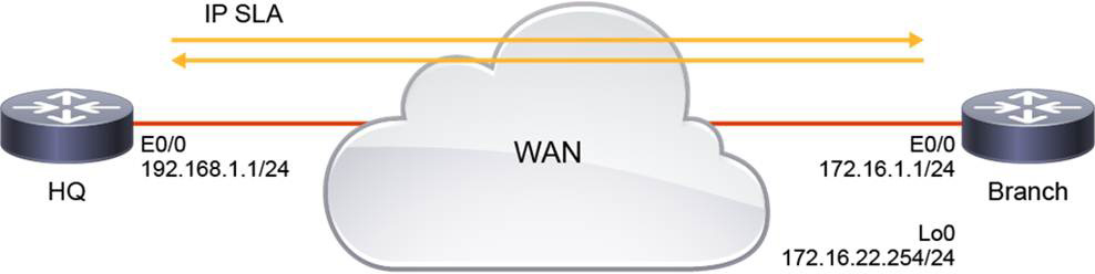
Figure 14-6 IP SLA Topology Example
Example 14-7 shows the commands used to configure both IP SLAs.
Example 14-7 Configuring Cisco IOS IP SLAs
HQ
ip sla 1
 icmp-echo 172.16.22.254
ip sla schedule 1 life forever start-time now
ip sla 2
 udp-jitter 172.16.22.254 65051 num-packets 20 interval 15
 request-data-size 160
 frequency 30
ip sla schedule 2 start-time now
Branch
ip sla responder
HQ# show ip sla summary
IPSLAs Latest Operation Summary
Codes: * active, ^ inactive, ~ pending

ID           Type        Destination       Stats       Return     Last
                                           (ms)        Code       Run
-----------------------------------------------------------------------
*1           icmp-echo   172.16.2.2        RTT=2       OK         50 seconds ago

*2           udp-jitter  172.16.2.2        RTT=1       OK         2 seconds ago


HQ# show ip sla statistics
IPSLAs Latest Operation Statistics

IPSLA operation id: 1
        Latest RTT: 3 milliseconds
Latest operation start time: 07:15:13 UTC Tue Jun 9 2020
Latest operation return code: OK
Number of successes: 10
Number of failures: 0
Operation time to live: Forever

IPSLA operation id: 2
Type of operation: udp-jitter
        Latest RTT: 1 milliseconds
Latest operation start time: 07:15:31 UTC Tue Jun 9 2020
Latest operation return code: OK
RTT Values:
        Number Of RTT: 20               RTT Min/Avg/Max: 1/1/4 milliseconds
Latency one-way time:
        Number of Latency one-way Samples: 19
        Source to Destination Latency one way Min/Avg/Max: 0/1/3 milliseconds
        Destination to Source Latency one way Min/Avg/Max: 0/0/1 milliseconds
Jitter Time:
        Number of SD Jitter Samples: 19
        Number of DS Jitter Samples: 19
        Source to Destination Jitter Min/Avg/Max: 0/1/3 milliseconds
        Destination to Source Jitter Min/Avg/Max: 0/1/1 milliseconds
<. . . output omitted . . .>
In the example, HQ is configured with two SLAs using the ip sla operation-number command. SLA number 1 is configured to send ICMP echo-request messages to the Loopback 0 IP address of the Branch router. IP SLA number 2 is configured for the same destination but has extra parameters: The destination UDP port is set to 65051, and every 30 seconds HQ will transmit 20 160-byte packets, which will be sent 15 milliseconds apart.
Both SLAs are then activated using the ip sla schedule command. The ip sla schedule command schedules when the test starts, how long it runs, and how long the collected data is kept. The syntax is as follows:
Router(config)# ip sla schedule operation-number [life {forever | seconds}] [start-time {hh:MM[:ss] [month day | day month] | pending | now | after hh:mm:ss}] [ageout seconds] [recurring]
With the life keyword, you set how long the IP SLA test runs. If you choose forever, the test runs until you manually remove it. By default, the IP SLA test runs for 1 hour.
With the start-time keyword, you set when the IP SLA test should start. You can start the test right away by issuing the now keyword, or you can configure a delayed start.
With the ageout keyword, you can control how long the collected data is kept.
With the recurring keyword, you can schedule a test to run periodically—for example, at the same time each day.
The Branch router is configured as an IP SLA responder. This is not required for SLA number 1, but it is required for SLA number 2.
You can use the show ip sla summary and show ip sla statistics commands to investigate the results of the tests. In this case, both SLAs are reporting an Ok status, and the UDP jitter SLA is gathering latency and jitter times between the HQ and Branch routers.
The IP SLA UDP jitter operation was designed primarily to diagnose network suitability for real-time traffic applications such as VoIP, video over IP, and real-time conferencing.
Jitter defines inter-packet delay variance. When multiple packets are sent consecutively from the source to the destination 10 milliseconds apart (for example), and the network is behaving ideally, the destination should receive the packets 10 milliseconds apart. But if there are delays in the network (such as queuing, arriving through alternate routes, and so on), the arrival delay between packets might be greater than or less than 10 milliseconds.
Switched Port Analyzer Overview
A traffic sniffer can be a valuable tool for monitoring and troubleshooting a network. Properly placing a traffic sniffer to capture a traffic flow but not interrupt it can be challenging.
When LANs were based on hubs, connecting a traffic sniffer was simple. When a hub receives a packet on one port, the hub sends out a copy of that packet on all ports except the one where the hub received the packet. A traffic sniffer that connected a hub port could thus receive all traffic in the network.
Modern local networks are essentially switched networks. After a switch boots, it starts to build up a Layer 2 forwarding table that is based on the source MAC address of the different packets that the switch receives. After this forwarding table is built, the switch forwards traffic destined for a MAC address directly to the corresponding port, thus preventing a traffic sniffer that is connected to another port from receiving the unicast traffic. The SPAN feature was therefore introduced on switches.
SPAN involves two different port types. The source port is a port that is monitored for traffic analysis. SPAN can copy ingress, egress, or both types of traffic from a source port. Both Layer 2 and Layer 3 ports can be configured as SPAN source ports. The traffic is copied to the destination (also called monitor) port.
The association of source ports and a destination port is called a SPAN session. In a single session, you can monitor at least one source port. Depending on the switch series, you might be able to copy session traffic to more than one destination port.
Alternatively, you can specify a source VLAN, where all ports in the source VLAN become sources of SPAN traffic. Each SPAN session can have either ports or VLANs as sources, but not both.
Local SPAN
A local SPAN session is an association of a source ports and source VLANs with one or more destination ports. You can configure local SPAN on a single switch. Local SPAN does not have separate source and destination sessions.
The SPAN feature allows you to instruct a switch to send copies of packets that are seen on one port to another port on the same switch.
To analyze the traffic flowing from PC1 to PC2, you need to specify a source port, as illustrated in Figure 14-7. You can either configure the GigabitEthernet0/1 interface to capture the ingress traffic or the GigabitEthernet0/2 interface to capture the egress traffic. Then you specify the GigabitEthernet0/3 interface as a destination port. Traffic that flows from PC1 to PC2 is then copied to that interface, and you can analyze it with a traffic sniffer such as Wireshark or SolarWinds.

Figure 14-7 Local SPAN Example
Besides monitoring traffic on ports, you can also monitor traffic on VLANs.
Local SPAN Configuration
To configure local SPAN, associate the SPAN session number with source ports or VLANs and associate the SPAN session number with the destination, as shown in the following configuration:
SW1(config)# monitor session 1 source interface Gigabit0/1
SW1(config)# monitor session 1 destination interface Gigabit0/3
This example configures the GigabitEthernet 0/1 interface as the source and the GigabitEthernet 0/3 interface as the destination of SPAN session 1.
When you configure the SPAN feature, you must know the following:
• The destination port cannot be a source port or vice versa.
• The number of destination ports is platform dependent; some platforms allow for more than one destination port.
• The destination port is no longer a normal switch port; only monitored traffic passes through that port.
In the previous example, the objective is to capture all the traffic that is sent or received by the PC connected to the GigabitEthernet 0/1 port on the switch. A packet sniffer is connected to the GigabitEthernet 0/3 port. The switch is instructed to copy all the traffic that it sends and receives on GigabitEthernet 0/1 to GigabitEthernet 0/3 by configuring a SPAN session.
If you do not specify a traffic direction, the source interface sends both transmitted (Tx) and received (Rx) traffic to the destination port to be monitored. You have the ability to specify the following options:
• Rx: Monitor received traffic.
• Tx: Monitor transmitted traffic.
• Both: Monitor both received and transmitted traffic (default).
Verify the Local SPAN Configuration
You can verify the configuration of a SPAN session by using the show monitor command, as illustrated in Example 14-8:
Example 14-8 Verifying Local SPAN
SW1# show monitor
Session 1
------------
Type                    : Local Session
Source ports            :
  Both                  : Gi0/1
Destination ports       : Gi0/3
  Encapsulation         : Native
     Ingress  :  Disabled
As shown in this example, the show monitor command returns the type of the session, the source ports for each traffic direction, and the destination port. In the example, information about session number 1 is presented: The source port for both traffic directions is GigabitEthernet 0/1, and the destination port is GigabitEthernet 0/3. The ingress SPAN is disabled on the destination port, so only traffic that leaves the switch is copied to it.
If you have more than one session configured, information about all sessions is shown after you use the show monitor command.
Remote SPAN
The local SPAN feature is limited because it allows for only a local copy on a single switch. A typical switched network usually consists of multiple switches, and it is possible to monitor ports spread all over the switched network with a single packet sniffer. This setup is possible with Remote Span (RSPAN).
Remote SPAN supports source and destination ports on different switches, and local SPAN supports only source and destination ports on the same switch. RSPAN consists of the RSPAN source session, RSPAN VLAN, and RSPAN destination session, as illustrated in Figure 14-8.

Figure 14-8 RSPAN
You separately configure the RSPAN source sessions and destination sessions on different switches. Your monitored traffic is flooded into an RSPAN VLAN that is dedicated for the RSPAN session in all participating switches. The RSPAN destination port can then be anywhere in that VLAN.
On some of the platforms, a reflector port needs to be specified together with an RSPAN VLAN. The reflector port is a physical interface that acts as a loopback and reflects the traffic that is copied from source ports to an RSPAN VLAN. No traffic is actually sent out of the interface that is assigned as the reflector port. The need for a reflector port is related to a hardware design limitation on some platforms. The reflector port can be used for only one session at a time. RSPAN supports source ports, source VLANs, and destinations on different switches, which provide remote monitoring of multiple switches across a network. RSPAN uses a Layer 2 VLAN to carry SPAN traffic between switches, which means there needs to be Layer 2 connectivity between the source and destination switches.
RSPAN Configuration
There are some differences between the configuration of RSPAN and the configuration of local SPAN. Example 14-9 shows the configuration of RSPAN. VLAN 100 is configured as the SPAN VLAN on SW1 and SW2. For SW1, the interface GigabitEthernet 0/1 is the source port in session 2, and VLAN 100 is the destination in session 2. For SW2, the interface GigabitEthernet 0/2 is the destination port in session 3, and VLAN 100 as the source in session 3. Session numbers are local to each switch, so they do not need to be the same on every switch.
Example 14-9 Configuring RSPAN
SW1(config)# vlan 100
SW1(config-vlan)# name SPAN-VLAN
SW1(config-vlan)# remote-span
SW1(config)# monitor session 2 source interface Gig0/1
SW1(config)# monitor session 2 destination remote vlan 100

SW2(config)# vlan 100
SW2(config-vlan)# name SPAN-VLAN
SW2(config-vlan)# remote-span
SW2(config)# monitor session 3 destination interface Gig0/2
SW2(config)# monitor session 3 source remote vlan 100
Figure 14-9 illustrates the topology for this example.
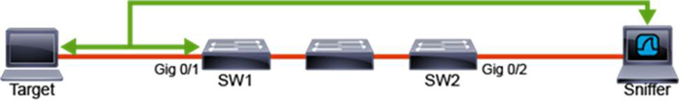
Figure 14-9 RSPAN Topology Example
Because the ports are now on two different switches, you use a special RSPAN VLAN to transport the traffic from one switch to the other. You configure this VLAN as you would any other VLAN, but you also enter the remote-span keyword in VLAN configuration mode. You need to define this VLAN on all switches in the path.
Verify the Remote SPAN Configuration
As with the local SPAN configuration, you can verify the RSPAN session configuration by using the show monitor command.
The only difference is that on the source switch, the session type is now identified as "Remote Source Session," while on the destination switch the type is marked as "Remote Destination Session," as shown in Example 14-10:
Example 14-10 Verifying Remote SPAN
SW1# show monitor
Session 2
------------
Type                    : Remote Source Session
Source ports            :
  Both                  : Gi0/1
Dest RSPAN VLAN         : 100


SW2# show monitor
Session 3
------------
Type                    : Remote Destination Session
Source RSPAN VLAN       : 100
Destination ports       : Gi0/2
  Encapsulation         : Native
     Ingress  :  Disabled
Encapsulated Remote SPAN
The Cisco-proprietary Encapsulated Remote SPAN (ERSPAN) mirrors traffic on one or more “source” ports and delivers the mirrored traffic to one or more “destination” ports on another switch. The traffic is encapsulated in Generic Routing Encapsulation (GRE) and is, therefore, routable across a Layer 3 network between the “source” switch and the “destination” switch. ERSPAN supports source ports, source VLANs, and destination ports on different switches, which provide remote monitoring of multiple switches across your network.
ERSPAN consists of an ERSPAN source session, routable ERSPAN GRE encapsulated traffic, and an ERSPAN destination session.
A device that has only an ERSPAN source session configured is called an ERSPAN source device, and a device that has only an ERSPAN destination session configured is called an ERSPAN termination device.
You separately configure ERSPAN source sessions and destination sessions on different switches.
To configure an ERSPAN source session on one switch, you associate a set of source ports or VLANs with a destination IP address, ERSPAN ID number, and, optionally, a VRF name. To configure an ERSPAN destination session on another switch, you associate the destinations with the source IP address, ERSPAN ID number, and, optionally, a virtual routing and forwarding (VRF) name.
ERSPAN source sessions do not copy locally sourced RSPAN VLAN traffic from source trunk ports that carry RSPAN VLANs. ERSPAN source sessions do not copy locally sourced ERSPAN GRE-encapsulated traffic from source ports. Each ERSPAN source session can have either ports or VLANs as sources but not both. The ERSPAN source session copies traffic from the source ports or source VLANs and forwards the traffic using routable GRE-encapsulated packets to the ERSPAN destination session. The ERSPAN destination session switches the traffic to the destinations.
ERSPAN Configuration
The diagram in Figure 14-10 shows the configuration of ERSPAN session 1 between Switch-1 and Switch-2.
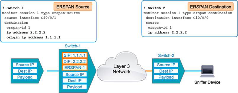
Figure 14-10 ERSPAN Configuration Example
On Switch-1, the source interface command associates the ERSPAN source session number with the source ports or VLANs and selects the traffic direction to be monitored. The destination command enters the ERSPAN source session destination configuration mode. erspan-id configures the ID number used by the source and destination sessions to identify the ERSPAN traffic, which must also be entered in the ERSPAN destination session configuration. The ip address command configures the ERSPAN flow destination IP address, which must also be configured on an interface on the destination switch and must be entered in the ERSPAN destination session configuration. The origin ip address command configures the IP address used as the source of the ERSPAN traffic.
On Switch-2, the destination interface command associates the ERSPAN destination session number with the destinations. The source command enters ERSPAN destination session source configuration mode. erspan-id configures the ID number used by the destination and destination sessions to identify the ERSPAN traffic. This must match the ID entered in the ERSPAN source session. The ip address command configures the ERSPAN flow destination IP address. This must be an address on a local interface and must match the address that entered in the ERSPAN source session.
ERSPAN Verification
You can use the show monitor session command to verify the configuration, as shown in Example 14-11:
Example 14-11 Verifying ERSPAN
Switch-1# show monitor session 1
Session 1
---------
Type                   : ERSPAN Source Session
Status                 : Admin Enabled
Source Ports           :
    RX Only            : Gi0/0/1
Destination IP Address : 2.2.2.2
MTU                    : 1464
Destination ERSPAN ID  : 1
Origin IP Address      : 1.1.1.1
Study Resources
For today’s exam topics, refer to the following resources for more study.