5

Graph Algorithms

Graphs offer a distinct way to represent data structures, especially when compared to structured or tabular data. While structured data, such as databases, excel at storing and querying static, uniform information, graphs shine in capturing intricate relationships and patterns that exist among entities. Think of Facebook, where every user is a node, and each friendship or interaction becomes a connecting edge; this web of connections can be best represented and analyzed using graph structures.

In the computational realm, certain problems, often those involving relationships and connections, are more naturally addressed using graph algorithms. At their core, these algorithms aim to understand the structure of the graph. This understanding involves figuring out how data points (or nodes) connect via links (or edges) and how to effectively navigate these connections to retrieve or analyze the desired data.

In this chapter, we’ll embark on a journey through the following territories:

• Graph representations: Various ways to capture graphs.
• Network theory analysis: The foundational theory behind network structures.
• Graph traversals: Techniques to efficiently navigate through a graph.
• Case study: Delving into fraud analytics using graph algorithms.
• Neighborhood techniques: Methods to ascertain and analyze localized regions within larger graphs.

Upon completion, we will have a robust grasp of graphs as data structures. We should be able to formulate complex relationships—both direct and indirect—and will be equipped to tackle complex, real-world problems using graph algorithms.

Understanding graphs: a brief introduction

In the vast interconnected landscapes of modern data, beyond the confines of tabular models, graph structures emerge as powerful tools to encapsulate intricate relationships. Their rise isn’t merely a trend but a response to challenges posed by the digital world’s interwoven fabric. Historical strides in graph theory, like Leonhard Euler’s pioneering solution to the Seven Bridges of Königsberg problem, laid the foundation for understanding complex relationships. Euler’s method of translating real-world issues into graphical representations revolutionized how we perceive and navigate graphs.

Graphs: the backbone of modern data networks

Graphs not only provide the backbone for platforms such as social media networks and recommendation engines but also serve as the key to unlocking patterns in seemingly unrelated sectors, like road networks, electrical circuits, organic molecules, ecosystems, and even the flow of logic in computer programs. What’s pivotal to graphs is their intrinsic capability to express both tangible and intangible interactions.

But why is this structure, with its nodes and edges, so central to modern computing? The answer lies in graph algorithms. Tailored for understanding and interpreting relationships, these mathematical algorithms are precisely designed to process connections. They establish clear steps to decode a graph, revealing both its overarching characteristics and intricate details.

Before delving into representations of graphs, it’s crucial to establish a foundational understanding of the mechanics behind them. Graphs, rooted in the rich soil of mathematics and computer science, offer an illustrative method to depict relationships among entities.

Real-world applications

The increasingly intricate patterns and connections observed in modern data find clarity in graph theory. Beyond the simple nodes and edges lie the solutions to some of the world’s most complex problems. When the mathematical precision of graph algorithms meets real-world challenges, the outcomes can be astonishingly transformative:

• Fraud detection: In the world of digital finance, fraudulent transactions can be deeply interconnected, often weaving a subtle web meant to deceive conventional detection systems. Graph theory is deployed to spot these patterns. For instance, a sudden spike in interconnected small transactions from a singular source to multiple accounts might be a hint at money laundering.

  By charting out these transactions on a graph, analysts can identify unusual patterns, isolate suspicious nodes, and trace the origin of potential fraud, ensuring that digital economies remain secure.

• Air traffic control: The skies are bustling with movement. Every aircraft must navigate a maze of routes while ensuring safe distances from others. Graph algorithms map the skies, treating each aircraft as a node and their flight paths as edges. The 2010 US air travel congestion events are a testament to the power of graph analytics. Scientists used graph theory to decipher systemic cascading delays, offering insights to optimize flight schedules and reduce the chances of such occurrences in the future.
• Disease spread modeling: The proliferation of diseases, especially contagious ones, doesn’t happen randomly; they follow the invisible lines of human interaction and movement. Graph theory creates intricate models that mimic these patterns. By treating individuals as nodes and their interactions as edges, epidemiologists have successfully projected disease spread, identifying potential hotspots and enabling timely interventions. For instance, during the early days of the COVID-19 pandemic, graph algorithms played a pivotal role in predicting potential outbreak clusters, helping to guide lockdowns and other preventive measures.
• Social media recommendations: Ever wondered how platforms like Facebook or Twitter suggest friends or content? Underlying these suggestions are vast graphs representing user interactions, interests, and behaviors. For example, if two users have multiple mutual friends or similar engagement patterns, there’s a high likelihood they might know each other or have aligned interests. Graph algorithms help decode these connections, enabling platforms to enhance user experience through relevant recommendations.

The basics of a graph: vertices (or nodes)

These are the individual entities or data points in the graph. Imagine each friend on your Facebook list as a separate vertex:

• Edges (or links): The connections or relationships between the vertices. When you become friends with someone on Facebook, an edge is formed between your vertex and theirs.
• Network: A larger structure formed by the interconnected web of vertices and edges. For example, the entirety of Facebook, with all its users and their friendships, can be viewed as a colossal network.

In Figure 5.1, A, B, and C represent vertices, while the lines connecting them are edges. It’s a simple representation of a graph, laying the groundwork for the more intricate structures and operations we’ll explore.

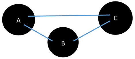
Figure 5.1: Graphic representation of a simple graph

Graph theory and network analysis

Graph theory and network analysis, although intertwined, serve different functions in understanding complex systems. While graph theory is a branch of discrete mathematics that provides the foundational concepts of nodes (entities) and edges (relationships), network analysis is the application of these principles to study and interpret real-world networks. For instance, graph theory might define the structure of a social media platform where individuals are nodes and their friendships are edges; conversely, network analysis would delve into this structure to uncover patterns, like influencer hubs or isolated communities, thereby providing actionable insights into user behavior and platform dynamics.

We will first start by looking into how we can mathematically and visually represent the graphs. Then we’ll harness the power of network analysis on these representations using a pivotal set of tools known as “graph algorithms.”

Representations of graphs

A graph is a structure that represents data in terms of vertices and edges. A graph is represented as a_Graph = (, ), where represents a set of vertices and represents a set of edges. Note that a_Graph has vertices and edges. It’s important to note that unless specified otherwise, an edge can be bidirectional, implying a two-way relationship between the connected vertices.

A vertex, , represents a real-world object, such as a person, a computer, or an activity. An edge, , connects two vertices in a network:

The preceding equation indicates that in a graph, all edges belong to a set, , and all vertices belong to a set, . Note that the notation ‘|’ used here is a symbolic representation indicating that an element belongs to a particular set, ensuring clarity in the relationship between edges, vertices, and their respective sets.

A vertex symbolizes tangible entities like individuals or computers, whereas an edge, connecting two vertices, denotes a relationship. Such relationships can be friendships between individuals, online connections, physical links between devices, or participatory connections such as attending a conference.

Graph mechanics and types

There are multiple types of graphs, each with its unique attributes:

• Simple graph: A graph with no parallel edges or loops.
• Directed graph (DiGraph): A graph where each edge has a direction, indicating a one-way relationship.
• Undirected graph: A graph where edges don’t have a specific direction, suggesting a mutual relationship.
• Weighted graph: A graph where each edge carries a weight, often representing distances, costs, etc.

In this chapter, we will use the networkx Python package to represent graphs. It can be downloaded from https://networkx.org/. Let’s try to create a simple graph using the networtx package in Python. A “simple graph,” as alluded to in graph theory, is a graph that has no parallel edges or loops. To begin with, let’s try to create an empty graph, aGraph, with no vertex or node:

import networkx as nx
graph = nx.Graph()

Let’s add a single vertex:

graph.add_node("Mike")

We can also add a series of vertices using a list:

graph.add_nodes_from(["Amine", "Wassim", "Nick"])

We can also add one edge between the existing vertices, as shown here:

graph.add_edge("Mike", "Amine")

Let’s now print the edges and avertices:

print(graph.nodes())
print(graph.edges())

['Mike', 'Amine', 'Wassim', 'Nick']
[('Mike', 'Amine')]

Please note that if we add an edge, this also leads to adding the associated vertices, if they do not already exist, as shown here:

G.add_edge("Amine", "Imran")

If we print the list of nodes, the following is the output that we observe:

print(graph.edges())

[('Mike', 'Amine'), ('Amine', 'Imran')]

Note that the request to add a vertex that already exists is silently ignored. The request is ignored or considered based on the type of graph we have created.

Ego-centered networks

At the heart of many network analyses lies a concept called the ego-centered network, or simply, the egonet. Imagine wanting to study not just an individual node but also its immediate surroundings. This is where the egonet comes into play.

Basics of egonets

For a given vertex—let’s call it m—the surrounding nodes that are directly connected to m from its direct neighborhood. This neighborhood, combined with m itself, constitutes the egonet of m. In this context:

• m is referred to as the ego.
• The directly connected nodes are termed one-hop neighbors or simply alters.

One-hop, two-hop, and beyond

When we say “one-hop neighbors,” we refer to nodes that are directly connected to our node of interest. Think of it as a single step or “hop” from one node to the next. If we were to consider nodes that are two steps away, they’d be termed “two-hop neighbors,” and so on. This nomenclature can extend to any number of hops, paving the way to understanding n-degree neighborhoods.

The ego network of a particular node, 3, is shown in the following graph:

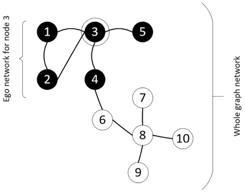
Figure 5.2: Egonet of node 3, showcasing the ego and its one-hop neighbors

Applications of egonets

Egonets are widely utilized in social network analysis. They are pivotal in understanding local structures in large networks and can offer insights into individual behaviors, based on their immediate network surroundings.

For instance, in online social platforms, egonets can help detect influential nodes or understand information dissemination patterns within localized network regions.

Introducing network analysis theory

Network analysis allows us to delve into data that’s interconnected, presenting it in the form of a network. It involves studying and employing methodologies to examine data that’s arranged in this network format. Here, we’ll break down the core elements and concepts related to network analysis.

At the heart of a network lies the “vertex,” serving as the fundamental unit. Picture a network as a web; vertices are the points of this web, while the links connecting them represent relationships between different entities under study. Notably, different relationships can exist between two vertices, implying that edges can be labeled to denote various kinds of relationships. Imagine two people being connected as “friends” and “colleagues”; both are different relationships but link the same individuals.

To fully harness the potential of network analysis, it’s vital to gauge the significance of a vertex within a network, especially concerning the problem at hand. Multiple techniques exist to aid us in ascertaining this significance.

Let’s look at some of the important concepts used in network analysis theory.

Understanding the shortest path

In graph theory, a “path” is defined as a sequence of nodes, connecting a starting node to an ending node, without revisiting any node in between. Essentially, a path outlines the route between two chosen vertices. The “length” of this path is determined by counting the number of edges it contains. Among the various paths possible between two nodes, the one with the least number of edges is termed the “shortest path.”

Identifying the shortest path is a fundamental task in many graph algorithms. However, its determination isn’t always straightforward. Over time, multiple algorithms have been developed to tackle this problem, with Dijkstra’s algorithm, introduced in the late 1950s, being one of the most renowned. This algorithm is designed to pinpoint the shortest distance in a graph and has found its way into applications like GPS devices, which rely on it to deduce the minimal distance between two points. In the realm of network routing, Dijkstra’s method again proves invaluable.

Big tech companies like Google and Apple are in a continuous race, especially when it comes to enhancing their map services. The goal is not just to identify the shortest route but to do so swiftly, often in mere seconds.

Later in this chapter, we’ll explore the breadth-first search (BFS) algorithm, a method that can serve as a foundation for Dijkstra’s algorithm. The standard BFS assumes equal costs to traverse any path in a graph. However, Dijkstra’s takes into account varying traversal costs. To adapt BFS into Dijkstra’s, we need to integrate these varying traversal costs.

Lastly, while Dijkstra’s algorithm focuses on identifying the shortest path from a single source to all other vertices, if one aims to determine the shortest paths between every pair of vertices in a graph, the Floyd-Warshall algorithm is more suitable.

Creating a neighborhood

When diving into graph algorithms, the term “neighborhood” frequently emerges. So, what do we imply by a neighborhood in this setting? Think of it as a close-knit community centered around a specific node. This “community” comprises nodes that either have a direct connection or are closely associated with the focal node.

As an analogy, envision a city map where landmarks represent nodes. The landmarks in the immediate vicinity of a notable place form its “neighborhood.”

A widely adopted approach to demarcate these neighborhoods is through the k-order strategy. Here, we determine a node’s neighborhood by pinpointing vertices that lie k hops away. For a hands-on understanding, at k=1, the neighborhood houses all nodes linked directly to the focal node. For k=2, it broadens to include nodes connected to these immediate neighbors, and the pattern continues.

Imagine a central dot within a circle as our target vertex. At k=1, any dot connected directly to this central figure is its neighbor. As we increment k the circle’s radius grows, encapsulating dots situated further away.

Harnessing and interpreting neighborhoods is important for graph algorithms, as it identifies key analysis zones.

Let’s look at the various criteria to create neighborhoods:

1. Triangles
2. Density

Let us look into them in more detail.

Triangles

In the expansive world of graph theory, pinpointing vertices that share robust interconnections can unveil critical insights. A classic approach is to spot triangles— subgraphs where three nodes maintain direct connections among themselves.

Let’s explore this through a tangible use case, fraud detection, which we’ll dissect in more detail in this chapter’s case study. Imagine a scenario where there’s an interconnected web – an “egonet” – revolving around a central person—let’s name him Max. In this egonet, apart from Max, there are two individuals, Alice and Bob. Now, this trio forms a “triangle” - Max is our primary figure (or “ego”), while Alice and Bob are the secondary figures (or “alters”).

Here’s where it gets interesting: if Alice and Bob have past records of fraudulent activities, it raises red flags about Max’s credibility. It’s like discovering two of your close friends have been involved in dubious deeds - it naturally puts you under scrutiny. However, if only one of them has a questionable past, then Max’s situation becomes ambiguous. We can’t label him outright but would need deeper investigation.

To visualize, picture Max at the center of a triangle, with Alice and Bob at the other vertices. Their interrelationships, especially if they carry negative connotations, can influence the perception of Max’s integrity.

Density

In the realm of graph theory, density is a metric that quantifies how closely knit a network is. Specifically, it’s the ratio of the number of edges present in the graph to the maximum possible number of edges. Mathematically, for a simple undirected graph, density is defined as:

To put this into perspective, let’s consider an example:

Suppose we are part of a book club with five members: Alice, Bob, Charlie, Dave, and Eve. If every member knows and has interacted with every other member, there would be a total of 10 connections (or edges) among them (Alice-Bob, Alice-Charlie, Alice-Dave, Alice-Eve, Bob-Charlie, and so on). In this case, the maximum number of possible connections or edges is 10. If all these connections exist, then the density is:

This indicates a perfectly dense or fully connected network.

However, let’s assume Alice knows only Bob and Charlie, Bob knows Alice and Dave, and Charlie knows only Alice. Dave and Eve, although members, haven’t interacted with anyone yet. In this scenario, there are only three actual connections: Alice-Bob, Alice-Charlie, and Bob-Dave. Let’s calculate the density:

This value, being less than 1, shows that the book club’s interaction network isn’t fully connected; many potential interactions (edges) haven’t occurred yet.

In essence, a density close to 1 indicates a tightly connected network, while a value closer to 0 suggests sparse interactions. Understanding density can help in various scenarios, from analyzing social networks to optimizing infrastructure planning, by gauging how interconnected the elements of the system are.

Understanding centrality measures

Centrality measures offer a window into understanding the significance of individual nodes within a graph. Think of centrality to identify key players or hubs in a network. For instance, in a social setting, it can help pinpoint influencers or central figures that hold sway. In urban planning, centrality might indicate pivotal buildings or junctions that play a critical role in traffic flow or accessibility. Understanding centrality is essential because it reveals nodes that are crucial for the functioning, cohesion, or influence within a network.

The most employed centrality metrics in graph analysis encompass:

• Degree: Reflects the direct connections a node has.
• Betweenness: Indicates how often a node acts as a bridge along the shortest path between two other nodes.
• Closeness: Represents how close a node is to all other nodes in the network.
• Eigenvector: Measures a node’s influence based on the quality of its connections, not just the quantity.

Note that centrality measures apply to all graphs. As we know, graphs are a general representation of objects (vertices or nodes) and their relationships (edges), and centrality measures help identify the importance or influence of these nodes within the graph. Recall that networks are specific realizations or applications of graphs, often representing real-world systems like social networks, transportation systems, or communication networks. So, while the centrality measures discussed can be applied universally across all types of graphs, they are often highlighted in the context of networks due to their practical implications in understanding and optimizing real-world systems.

Let’s delve deeper into these metrics to better appreciate their utility and nuances.

Degree

The number of edges connected to a particular vertex is called its degree. It can indicate how well connected a particular vertex is and its ability to quickly spread a message across a network.

Let’s consider a_Graph = (, ), where represents a set of vertices and represents a set of edges. Recall that a_Graph has vertices and edges. If we divide the degree of a node by (), it is called degree centrality:

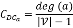
Now, let’s look at a specific example. Consider the following graph:

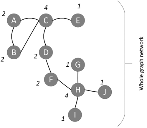
Figure 5.3: A sample graph illustrating the concept of degree and degree centrality

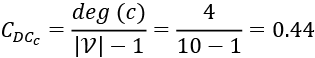
Now, in the preceding graph, vertex C has a degree of 4. Its degree centrality can be calculated as follows:

Betweenness

Betweenness centrality is a key measure that gauges the significance of a vertex within a graph. When applied to social media contexts, it assesses the likelihood that an individual plays a crucial role in communications within a specific subgroup. In terms of computer networks, where a vertex symbolizes a computer, betweenness offers insights into the potential impact on communications between nodes if a particular computer (or vertex) were to fail.

To calculate the betweenness of vertex a in a certain a_Graph = (, ), follow these steps:

1. Compute the shortest paths between each pair of vertices in a_Graph. Let’s represent this with
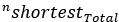
2. From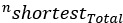, count the number of shortest paths that pass through vertex a. Let’s represent this with
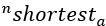
3. Calculate the betweenness with:

Fairness and closeness

In graph theory, we often want to determine how central or how distant a specific vertex is in relation to other vertices. One way to quantify this is by calculating a metric known as “fairness.” For a given vertex, say “a,” in a graph “g,” the fairness is determined by adding up the distances from vertex “a” to every other vertex in the graph. Essentially, it gives us a sense of how “spread out” or “far” a vertex is from its neighbors. This concept ties in closely with the idea of centrality, where the centrality of a vertex measures its overall distance from all other vertices.

Conversely, “closeness” can be thought of as the opposite of fairness. While it might be intuitive to think of closeness as the negative sum of a vertex’s distances from other vertices, that’s not technically accurate. Instead, closeness measures how near a vertex is to all other vertices in a graph, often calculated by taking the reciprocal of the sum of its distances to others.

Both fairness and closeness are essential metrics in network analysis. They provide insight into how information might flow within a network or how influential a particular node might be. By understanding these metrics, one can derive a deeper comprehension of network structures and their underlying dynamics.

Eigenvector centrality

Eigenvector centrality is a metric that evaluates the significance of nodes within a graph. Rather than just considering the number of direct connections a node has, it takes into account the quality of those connections. In simple terms, a node is considered important if it is connected to other nodes that are themselves significant within the network.

To give this a bit more mathematical context, imagine each node v has a centrality score x(v). For every node v, its eigenvector centrality is calculated based on the sum of the centrality scores of its neighbors, scaled by a factor (eigenvector’s associated eigenvalue):

where M(v) denotes the neighbors of v.

This idea of weighing the importance of a node based on its neighbors was foundational for Google when they developed the PageRank algorithm. The algorithm assigns a rank to every web page on the internet, signifying its importance, and is heavily influenced by the concept of eigenvector centrality.

For readers interested in our upcoming watchtower example, understanding the essence of eigenvector centrality will provide deeper insights into the workings of sophisticated network analysis techniques.

Calculating centrality metrics using Python

Let’s create a network and then try to calculate its centrality metrics.

1. Setting the foundation: libraries and data

This includes importing necessary libraries and defining our data:

import networkx as nx
import matplotlib.pyplot as plt

For our sample, we’ve considered a set of vertices and edges:

vertices = range(1, 10)
edges = [(7, 2), (2, 3), (7, 4), (4, 5), (7, 3), (7, 5), (1, 6), (1, 7), (2, 8), (2, 9)]

In this setup, vertices represent individual points or nodes in our network. The edges signify the relationships or links between these nodes.

2. Crafting the graph

With the foundation set, we proceed to craft our graph. This involves feeding our data (vertices and edges) into the graph structure:

graph = nx.Graph()
graph.add_nodes_from(vertices)
graph.add_edges_from(edges)

Here, the Graph() function initiates an empty graph. The subsequent methods, add_nodes_from and add_edges_from, populate this graph with our defined nodes and edges.

3. Painting a picture: visualizing the graph

A graphical representation often speaks louder than raw data. Visualization not only aids comprehension but also offers a snapshot of the graph’s overall structure:

nx.draw(graph, with_labels=True, node_color='y', node_size=800)
plt.show()

This code paints the graph for us. The with_labels=True method ensures each node is labeled, node_color provides a distinct color, and node_size adjusts the node’s size for clarity.

Figure 5.4: A schematic representation of the graph, showcasing nodes and their inter-relationships

Once our graph is established, the next pivotal step is to compute and understand the centrality measures of each node. Centrality measures, as previously discussed, gauge the importance of nodes in the network.

• Degree centrality: This measure gives the fraction of nodes that a particular node is connected to. In simpler terms, if a node has a high degree centrality, it’s connected to many other nodes in a graph. The function nx.degree_centrality(graph) returns a dictionary with nodes as keys and their respective degree centrality as values:

  print("Degree Centrality:", nx.degree_centrality(graph))
  

  Degree Centrality: {1: 0.25, 2: 0.5, 3: 0.25, 4: 0.25, 5: 0.25, 6: 0.125, 7: 0.625, 8: 0.125, 9: 0.125}
  
• Betweenness centrality: This metric indicates the number of shortest paths passing through a particular node. Nodes with high betweenness centrality can be seen as “bridges” or “bottlenecks” between different parts of a graph. The function nx.betweenness_centrality(graph) computes this for each node:

  print("Betweenness Centrality:", nx.betweenness_centrality(graph))
  

  Betweenness Centrality: {1: 0.25, 2: 0.46428571428571425, 3: 0.0, 4: 0.0, 5: 0.0, 6: 0.0, 7: 0.7142857142857142, 8: 0.0, 9: 0.0}
  
• Closeness centrality: This represents how close a node is to all other nodes in a graph. A node with high closeness centrality can quickly interact with all other nodes, making it centrally located. This measure is calculated with nx.closeness_centrality(graph):

  print("Closeness Centrality:", nx.closeness_centrality(graph))
  

  Closeness Centrality: {1: 0.5, 2: 0.6153846153846154, 3: 0.5333333333333333, 4: 0.47058823529411764, 5: 0.47058823529411764, 6: 0.34782608695652173, 7: 0.7272727272727273, 8: 0.4, 9: 0.4}
  
• Eigenvector centrality: Unlike the degree centrality, which counts direct connections, the eigenvector centrality considers the quality or strength of these connections. Nodes connected to other high-scoring nodes get a boost, making it a measure of influential nodes. We further sort these centrality values for ease of interpretation:

  eigenvector_centrality = nx.eigenvector_centrality(graph)
  sorted_centrality = sorted((vertex, '{:0.2f}'.format(centrality_val)) 
                             for vertex, centrality_val in eigenvector_centrality.items())
  print("Eigenvector Centrality:", sorted_centrality)
  

  Eigenvector Centrality: [(1, '0.24'), (2, '0.45'), (3, '0.36'), (4, '0.32'), (5, '0.32'), (6, '0.08'), (7, '0.59'), (8, '0.16'), (9, '0.16')]
  

Note that the metrics of centrality are expected to give the centrality measure of a particular vertex in a graph or subgraph. Looking at the graph, the vertex labeled 7 seems to have the most central location. Vertex 7 has the highest values in all four metrics of centrality, thus reflecting its importance in this context.

Now let’s look into how we can retrieve information from the graphs. Graphs are complex data structures with lots of information stored both in vertices and edges. Let’s look at some strategies that can be used to navigate through graphs efficiently, in order to gather information from them to answer queries.

Social network analysis

Social Network Analysis (SNA) stands out as a significant application within graph theory. At its core, an analysis qualifies as SNA when it adheres to the following criteria:

• Vertices in a graph symbolize individuals.
• Edges signify social connections between these individuals, which include friendships, shared interests, familial ties, differences in opinions, and more.
• The primary objective of graph analysis leans toward understanding a pronounced social context.

One intriguing facet of SNA is its capacity to shed light on patterns linked to criminal behavior. By mapping out relationships and interactions, it’s feasible to pinpoint patterns or anomalies that might indicate fraudulent activities or behaviors. For instance, analyzing the connectivity patterns might reveal unusual connections or frequent interactions in specific locations, hinting at potential criminal hotspots or networks.

Thus, SNA—due to its inherent distributed and interconnected architecture of social networks—is one of the most powerful use cases for graph theory. Another way to abstract a graph is by considering it as a network and applying an algorithm designed for networks. This whole area is called network analysis theory, which we will discuss next.

Understanding graph traversals

To make use of graphs, information needs to be mined from them. Graph traversal is defined as the strategy used to make sure that every vertex and edge is visited in an orderly manner. An effort is made to make sure that each vertex and edge is visited exactly once—no more and no less. Broadly, there can be two different ways of traveling a graph to search the data in it.

Earlier in this chapter we learned that going by breadth is called breadth-first search (BFS) – going by depth is called depth-first search (DFS). Let’s look at them one by one.

BFS

BFS works best when there is a concept of layers or levels of neighborhoods in the a_Graph we deal with. For example, when the connections of a person on LinkedIn are expressed as a graph, there are first-level connections and then there are second-level connections, which directly translate to the layers.

The BFS algorithm starts from a root vertex and explores the vertices in the neighborhood vertices. It then moves to the next neighborhood level and repeats the process.

Let’s look at a BFS algorithm. For that, let’s first consider the following undirected graph:

Figure 5.5: An undirected graph demonstrating personal connections

Constructing the adjacency list

In Python, the dictionary data structure lends itself conveniently to representing the adjacency list of a graph. Here’s how we can define an undirected graph:

graph={ 'Amin'   : {'Wasim', 'Nick', 'Mike'},
         'Wasim' : {'Imran', 'Amin'},
         'Imran' : {'Wasim','Faras'},
         'Faras' : {'Imran'},
         'Mike'  : {'Amin'},
         'Nick' :  {'Amin'}}

To implement it in Python, we will proceed as follows.

We will first explain the initialization and then the main loop.

BFS algorithm implementation

The algorithm implementation will involve two main phases: the initialization and the main loop.

Initialization

Our traversal through the graph relies on two key data structures:

• visited: A set that will hold all the vertices we’ve explored. It starts empty.
• queue: A list used to hold vertices pending exploration. Initially, it will contain just our starting vertex.

Main loop

The primary logic of BFS revolves around exploring nodes layer by layer:

1. Remove the first node from the queue and consider it as the current node for the iteration:

   node = queue.pop(0)
   
2. If the node hasn’t been visited, mark it as visited and fetch its neighbors:

   if node not in visited:
       visited.add(node)
       neighbours = graph[node]
   
3. Append unvisited neighbors to the queue:

   for neighbour in neighbours:
       if neighbour not in visited:
           queue.append(neighbour)
   
4. Once the main loop is complete, the visited data structure is returned, which contains all the nodes traversed.

Complete BFS code implementation

The complete code, with both initialization and the main loop, will be as follows:

def bfs(graph, start):
    visited = set()
    queue = [start]
    while queue:
        node = queue.pop(0)
        if node not in visited:
            visited.add(node)
            neighbours = graph[node]
            unvisited_neighbours = [neighbour for neighbour in neighbours                                     if neighbour not in visited]
            queue.extend(unvisited_neighbours)
   return visited

The BFS traversal mechanism is as follows:

1. The process starts at level one, represented by the node “Amin.”
2. It then expands to level two, visiting “Wasim’,” “Nick,” and “Mike.”
3. Subsequently, BFS delves into levels three and four, visiting “Imran” and “Faras,” respectively.

By the time BFS completes its traversal, all nodes have been accounted for in the visited set, and the queue is empty.

Using BFS for specific searches

To practically understand BFS in action, let’s use our implemented function to find a path to a specific person in our graph:

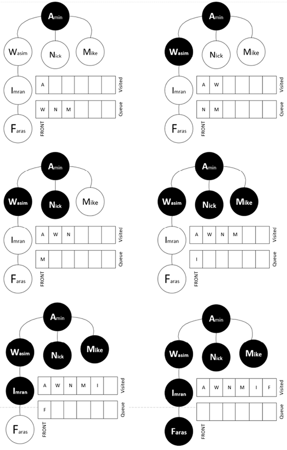
Figure 5.6: Layered traversal of a graph using BFS

Now, let’s try to find a specific person from this graph using BFS. Let’s specify the data that we are searching for and observe the results:

start_node = 'Amin'
print(bfs(graph, start_node))

{'Faras', 'Nick', 'Wasim', 'Imran', 'Amin', 'Mike'}

This signifies the sequence of nodes accessed when BFS starts from Amin.

Now let’s look into the DFS algorithm.

DFS

DFS offers an alternative approach to graph traversal than BFS. While BFS seeks to explore the graph level by level, focusing on immediate neighbors first, DFS ventures as deep as possible down a path before backtracking.

Imagine a tree. Starting from the root, DFS dives down to the furthest leaf on a branch, marks all nodes along that branch as visited, then backtracks to explore other branches in a similar manner. The idea is to reach the furthest leaf node on a given branch before considering other branches. “Leaf” is a term used to refer to nodes in a tree that don’t have any child nodes or, in a graph context, any unvisited adjacent nodes.

To ensure that the traversal doesn’t get stuck in a loop, especially in cyclic graphs, DFS employs a Boolean flag. This flag indicates whether a node has been visited, preventing the algorithm from revisiting nodes and getting trapped in infinite cycles.

To implement DFS, we will use a stack data structure, which was discussed in detail in Chapter 2, Data Structures Used in Algorithms. Remember that a stack is based on the Last In, First Out (LIFO) principle. This contrasts with a queue, as used for BFS, which works on the First In, First Out (FIFO) principle:

The following code is used for DFS:

def dfs(graph, start, visited=None):
    if visited is None:
        visited = set()
    visited.add(start)
    print(start)
    for next in graph[start] - visited:
        dfs(graph, next, visited)
    return visited

Let’s again use the following code to test the dfs function defined previously:

graph={ 'Amin' : {'Wasim', 'Nick', 'Mike'},
         'Wasim' : {'Imran', 'Amin'},
         'Imran' : {'Wasim','Faras'},
         'Faras' : {'Imran'},
         'Mike'  :{'Amin'},
         'Nick'  :{'Amin'}}

If we run this algorithm, the output will look like the following:

Amin
Wasim
Imran
Faras
Nick
Mike

Let’s look at the exhaustive traversal pattern of this graph using the DFS methodology:

1. The iteration starts from the top node, Amin.
2. Then, it moves to level two, Wasim. From there, it moves toward the lower levels until it reaches the end, which is the Imran and Fares nodes.
3. After completing the first full branch, it backtracks and then goes to level two to visit Nick and Mike.

The traversal pattern is shown in Figure 5.7:

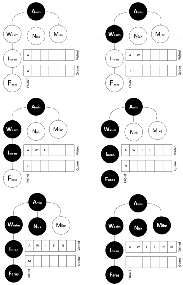
Figure 5.7: A visual representation of DFS traversal

Note that DFS can be used in trees as well.

Let’s now look at a case study, which explains how the concepts we have discussed so far in this chapter can be used to solve a real-world problem.

Case study: fraud detection using SNA

Introduction

Humans are inherently social, and their behavior often reflects the company they keep. In the realm of fraud analytics, a principle called “homophily” signifies the likelihood of individuals having associations based on shared attributes or behaviors. A homophilic network, for instance, might comprise people from the same hometown, university, or with shared hobbies. The underlying principle is that individuals’ behavior, including fraudulent activity, might be influenced by their immediate connections. This is also sometimes referred to as “guilt by association.”

What is fraud in this context?

In the context of this case study, fraud refers to deceptive activities that may include impersonation, credit card theft, fake check submission, or any other illicit activities that can be represented and analyzed in a network of relationships. In an effort to understand the process, let’s first look at a simple case. For that, let’s use a network with nine vertices and eight edges. In this network, four of the vertices are known fraud cases and are classified as fraud (F). Five of the remaining people have no fraud-related history and are classified as non-fraud (NF).

We will write code with the following steps to generate this graph:

1. Let’s import the packages that we need:

   import networkx as nx
   import matplotlib.pyplot as plt
   
2. Define the data structures of vertices and edges:

   vertices = range(1,10)
   edges= [(7,2), (2,3), (7,4), (4,5), (7,3), (7,5), (1,6),(1,7),(2,8),(2,9)]
   
3. Instantiate the graph:

   graph = nx.Graph()
   
4. Now, draw the graph:

   graph.add_nodes_from(vertices)
   graph.add_edges_from(edges)
   positions = nx.spring_layout(graph)
   
5. Let’s define the NF nodes:

   nx.draw_networkx_nodes(graph, positions, 
                          nodelist=[1, 4, 3, 8, 9], 
                          with_labels=True, 
                          node_color='g', 
                          node_size=1300)
   
6. Now, let’s create the nodes that are known to be involved in fraud:

   nx.draw_networkx_nodes(graph, positions, 
                          nodelist=[1, 4, 3, 8, 9], 
                          with_labels=True, 
                          node_color='g', 
                          node_size=1300)
   
7. Finally, create labels for the nodes:

   labels = {1: '1 NF', 2: '2 F', 3: '3 NF', 4: '4 NF', 5: '5 F', 6: '6 F', 7: '7 F', 8: '8 NF', 9: '9 NF'}
   nx.draw_networkx_labels(graph, positions, labels, font_size=16)
   nx.draw_networkx_edges(graph, positions, edges, width=3, alpha=0.5, edge_color='b')
   plt.show()
   

Once the preceding code runs, it will show us a graph like this:

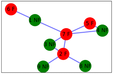
Figure 5.8: Initial network representation showing both fraudulent and non-fraudulent nodes

Note that we have already conducted a detailed analysis to classify each node as a graph or non-graph. Let’s assume that we add another vertex, named q, to the network, as shown in the following figure. We have no prior information about this person and whether this person is involved in fraud or not. We want to classify this person as NF or F based on their links to the existing members of the social network:

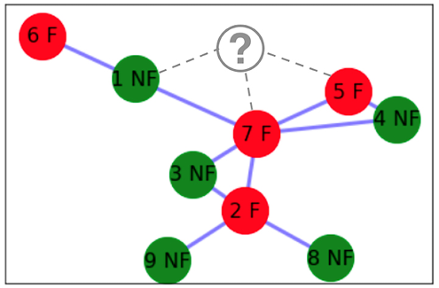
Figure 5.9: Introduction of a new node to the existing network

We have devised two ways to classify this new person, represented by node q, as F or NF:

• Using a simple method that does not use centrality metrics and additional information about the type of fraud
• Using a watchtower methodology, which is an advanced technique that uses the centrality metrics of the existing nodes, as well as additional information about the type of fraud

We will discuss each method in detail.

Conducting simple fraud analytics

The simple technique of fraud analytics is based on the assumption that in a network, the behavior of a person is affected by the people they are connected to. In a network, two vertices are more likely to have similar behavior if they are associated with each other.

Based on this assumption, we will devise a simple technique. If we want to find the probability that a certain node, a, belongs to F, the probability is represented by P(F/q) and is calculated as follows:

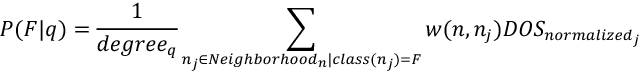
Let’s apply this to the preceding figure, where Neighborhood_n represents the neighborhood of vertex n and w(n, n_j) represents the weight of the connection between n and n_j. Also, DOS_normalized is the value of the degree of suspicion normalized between 0 and 1. Finally, degree_q is the degree of node q.

The probability is calculated as follows:

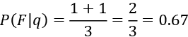
Based on this analysis, the likelihood of this person being involved in fraud is 67%. We need to set a threshold. If the threshold is 30%, then this person is above the threshold value, and we can safely flag them as F.

Note that this process needs to be repeated for each of the new nodes in the network.

Now, let’s look at an advanced way of conducting fraud analytics.

Presenting the watchtower fraud analytics methodology

The previous simple fraud analytics technique has the following two limitations:

• It does not evaluate the importance of each vertex in the social network. A connection to a hub that is involved in fraud may have different implications than a relationship with a remote, isolated person.
• When labeling someone as a known case of fraud in an existing network, we do not consider the severity of the crime.

The watchtower fraud analytics methodology addresses these two limitations. First, let’s look at a couple of concepts.

Scoring negative outcomes

If a person is known to be involved in fraud, we say that there is a negative outcome associated with this individual. Not every negative outcome is of the same severity or seriousness. A person known to be impersonating another person will have a more serious type of negative outcome associated with them, compared to someone who is just trying to use an expired $20 gift card in a creative way to make it valid.

From a score of 1 to 10, we will rate various negative outcomes as follows:

Note that these scores will be based on our analysis of fraud cases and their impact from historical data.

Degree of suspicion

The degree of suspicion (DOS) quantifies our level of suspicion that a person may be involved in fraud. A DOS value of 0 means that this is a low-risk person, and a DOS value of 9 means that this is a high-risk person.

Analysis of historical data shows that professional fraudsters have important positions in their social networks. To incorporate this, we first calculate all of the four centrality metrics of each vertex in our network. We then take the average of these vertices. This translates to the importance of that particular person in the network.

If a person associated with a vertex is involved in fraud, we illustrate this negative outcome by scoring the person using the pre-determined values shown in the preceding table. This is done so that the severity of the crime is reflected in the value of each individual DOS.

Finally, we multiply the average of the centrality metrics and the negative outcome score to get the value of the DOS. We normalize the DOS by dividing it by the maximum value of the DOS in the network.

Let’s calculate the DOS for each of the nine nodes in the previous network:

Each of the nodes and their normalized DOS is shown in the following figure:

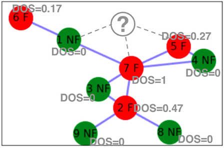
Figure 5.10: Visualization of nodes with their calculated DOS values

In order to calculate the DOS of the new node that has been added, we will use the following formula:

Using the relevant values, we will calculate the DOS as follows:

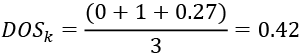
This will indicate the risk of fraud associated with this new node added to the system. It means that on a scale of 0 to 1, this person has a DOS value of 0.42. We can create different risk bins for the DOS, as follows:

Based on these criteria, it can be seen that the new individual is a high-risk person and should be flagged.

Usually, a time dimension is not involved when conducting such an analysis. But now, there are some advanced techniques that look at the growth of a graph as time progresses. This allows researchers to look at the relationship between vertices as the network evolves. Although such time-series analysis on graphs will increase the complexity of the problem many times over, it may give additional insight into the evidence of fraud that was not possible otherwise.

Summary

In this chapter, we learned about graph-based algorithms. This chapter used different techniques of representing, searching, and processing data represented as graphs. We also developed skills to be able to calculate the shortest distance between two vertices, and we built neighborhoods in our problem space. This knowledge should help us use graph theory to address problems such as fraud detection.

In the next chapter, we will focus on different unsupervised machine learning algorithms. Many of the use-case techniques discussed in this chapter complement unsupervised learning algorithms, which will be discussed in detail in the next chapter. Finding evidence of fraud in a dataset is an example of such use cases.

Learn more on Discord

To join the Discord community for this book – where you can share feedback, ask questions to the author, and learn about new releases – follow the QR code below:

https://packt.link/WHLel