8

Neural Network Algorithms

There is no algorithm for humor.

—Robert Mankoff

Neural networks have been a topic of investigation for over seven decades, but their adoption was restricted due to constraints in computational capabilities and the dearth of digitized data. Today’s environment is significantly altered due to our growing need to solve complex challenges, the explosive growth in data production, and advancements such as cloud computing, which provide us with impressive computational abilities. These enhancements have opened up the potential for us to develop and apply these sophisticated algorithms to solve complex problems that were previously deemed impractical. In fact, this is the research area that is rapidly evolving and is responsible for most of the major advances claimed by leading-edge tech fields such as robotics, edge computing, natural language processing, and self-driving cars.

This chapter first introduces the main concepts and components of a typical neural network. Then, it presents the various types of neural networks and explains the different kinds of activation functions used in these neural networks. Then, the backpropagation algorithm is discussed in detail, which is the most widely used algorithm for training a neural network. Next, the transfer learning technique is explained, which can be used to greatly simplify and partially automate the training of models. Finally, how to use deep learning to flag fraudulent documents by way of a real-world example application.

The following are the main concepts discussed in this chapter:

• Understanding neural networks
• The evolution of neural networks
• Training a neural network
• Tools and frameworks
• Transfer learning
• Case study: using deep learning for fraud detection

Let’s start by looking at the basics of neural networks.

The evolution of neural networks

A neural network, at its most fundamental level, is composed of individual units known as neurons. These neurons serve as the cornerstone of the neural network, with each neuron performing its own specific task. The true power of a neural network unfolds when these individual neurons are organized into structured layers, facilitating complex processing. Each neural network is composed of an intricate web of these layers, connected to create an interconnected network.

The information or signal is processed step by step as it travels through these layers. Each layer modifies the signal, contributing to the overall output. To explain, the initial layer receives the input signal, processes it, and then passes it to the next layer. This subsequent layer further processes the received signal and transfers it onward. This relay continues until the signal reaches the final layer, which generates the desired output.

It’s these hidden layers, or intermediate layers, that give neural networks their ability to perform deep learning. These layers create a hierarchy of abstract representations by transforming the raw input data progressively into a form that is more useful. This facilitates the extraction of higher-level features from the raw data.

This deep learning capability has a vast array of practical applications, from enabling Amazon’s Alexa to understand voice commands to powering Google’s Images and organizing Google Photos.

Historical background

Inspired by the workings of neurons in the human brain, the concept of neural networks was proposed by Frank Rosenblatt in 1957. To understand the architecture fully, it is helpful to briefly look at the layered structure of neurons in the human brain. (Refer to Figure 8.1 to get an idea of how the neurons in the human brain are linked together.)

In the human brain, dendrites act as sensors that detect a signal. Dendrites are integral components of a neuron, serving as the primary sensory apparatus. They are responsible for detecting incoming signals. The signal is then passed on to an axon, which is a long, slender projection of a nerve cell. The function of the axon is to transmit this signal to muscles, glands, and other neurons. As shown in the following diagram, the signal travels through interconnecting tissue called a synapse before being passed on to other neurons. Note that through this organic pipeline, the signal keeps traveling until it reaches the target muscle or gland, where it causes the required action. It typically takes seven to eight milliseconds for the signal to pass through the chain of neurons and reach its destination:

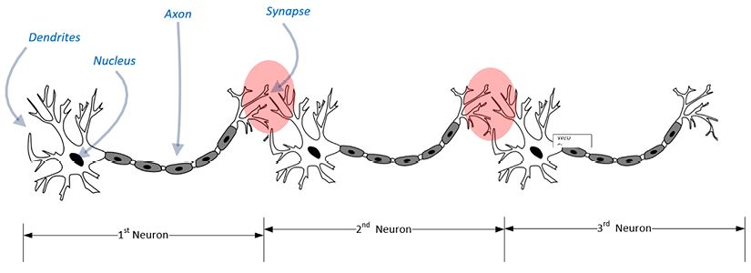
Figure 8.1: Neuron chained together in the human brain

Inspired by this natural architectural masterpiece of signal processing, Frank Rosenblatt devised a technique that would mean digital information could be processed in layers to solve a complex mathematical problem. His initial attempt at designing a neural network was quite simple and looked like a linear regression model. This simple neural network did not have any hidden layers and was named a perceptron. This simple neural network without any layers, the perceptron, became the basic unit for neural networks. Essentially, a perceptron is the mathematical analog of a biological neuron and hence, serves as the fundamental building block for more complex neural networks.

Now, let us delve into a concise historical account of the evolutionary journey of Artificial Intelligence (AI).

AI winter and the dawn of AI spring

The initial enthusiasm toward the groundbreaking concept of the perceptron soon faded when its significant limitations were discovered. In 1969, Marvin Minsky and Seymour Papert conducted an in-depth study that led to the revelation that the perceptron was restricted in its learning capabilities. They found that a perceptron was incapable of learning and processing complex logical functions, even struggling with simple logic functions such as XOR.

This discovery triggered a significant decline in interest in Machine Learning (ML) and neural networks, commencing an era often referred to as the “AI winter.” This was a period when the global research community largely dismissed the potential of AI, viewing it as inadequate for tackling complex problems.

On reflection, the “AI winter” was in part a consequence of the restrictive hardware capabilities of the time. The hardware either lacked the necessary computing power or was prohibitively expensive, which severely hampered advancements in AI. This limitation stymied the progress and application of AI, leading to widespread disillusionment in its potential.

Toward the end of the 1990s, there was a tidal shift regarding the image of AI and its perceived potential. The catalyst for this change was the advances in distributed computing, which provided easily available and affordable infrastructure. Seeing the potential, the newly crowned IT giants of that time (like Google) made AI the focus of their R&D efforts. The renewed interest in AI resulted in the thaw of the so-called AI winter. The thaw reinvigorated research in AI. This eventually resulted in turning the current era into an era that can be called the AI spring, where there is so much interest in AI and neural networks. Also, the digitized data was not available.

Understanding neural networks

First, let us start with the heart of the neural network, the perceptron. You can think of a single perceptron as the simplest possible neural network, and it forms the basic building block of modern complex multi-layered architectures. Let us start by understanding the working of a perceptron.

Understanding perceptrons

A single perceptron has several inputs and a single output that is controlled or activated by an activation function. This is shown in Figure 8.2:

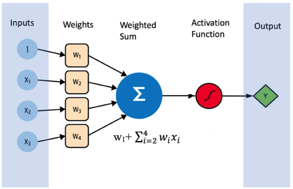
Figure 8.2: A simple perceptron

The perceptron shown in Figure 8.2 has three input features; x₁, x₂, and x₃. We also add a constant signal called bias. The bias plays a critical role in our neural network model, as it allows for flexibility in fitting the data. It operates similarly to an intercept added in a linear equation—acting as a sort of “shift” of the activation function—thereby allowing us to fit the data better when our inputs are equal to zero. The input features and the bias get multiplied by weights and are summed up as a weighted sum This weighted sum is passed on to the activation function, which generates the output y. The ability to use a wide variety of activation functions to formulate complex relationships between features and labels is one of the strengths of neural networks. A variety of activation functions is selectable through the hyperparameters. Some common examples include the sigmoid function, which squashes values between 0 and 1, making it a good choice for binary classification problems; the tanh function, which scales values between -1 and 1, providing a zero-centered output; and the Rectified Linear Unit (ReLU) function, which sets all negative values in the vector to zero, effectively removing any negative influence, and is commonly used in convolutional neural networks. These activation functions are discussed in detail later in the chapter.

Let us now look into the intuition behind neural networks.

Understanding the intuition behind neural networks

In the last chapter, we discussed some traditional ML algorithms. These traditional ML algorithms work great for many important use cases. But they do have limitations as well. When the underlying patterns in the training dataset begin to become non-linear and multidimensional, it starts to go beyond the capabilities of traditional ML algorithms to accurately capture the complex relationships between features and labels. These incomprehensive, somewhat simplistic mathematical formulations of complex patterns result in suboptimal performance of the trained models for these use cases.

In real-world scenarios, we often encounter situations where the relationships between our features and labels are not linear or straightforward but present complex patterns. This is where neural networks shine, offering us a powerful tool for modeling such intricacies.

Neural networks are particularly effective when dealing with high-dimensional data or when the relationships between features and the outcome are non-linear. For instance, they excel in applications like image and speech recognition, where the input data (pixels or sound waves) has complex, hierarchical structures. Traditional ML algorithms might struggle in these instances, given the high degree of complexity and the non-linear relationships between features.

While neural networks are incredibly powerful tools, it’s crucial to acknowledge that they aren’t without their limitations. These restrictions, explored in detail later in this chapter, are critical to grasp for the practical and effective use of neural networks in tackling real-world dilemmas.

Now, let’s illustrate some common patterns and their associated challenges when simpler ML algorithms like linear regression are employed. Picture this – we’re trying to predict a data scientist’s salary based on the “years spent in education.” We have collected two different datasets from two separate organizations.

First, let’s introduce you to Dataset 1, illustrated in Figure 8.3(a). It depicts a relatively straightforward relationship between the feature (years spent in education) and the label (salary), which appears to be linear. However, even this simple pattern throws a couple of challenges when we attempt to mathematically model it using a linear algorithm:

• We know that a salary cannot be negative, meaning that regardless of the years spent in education, the salary (y) should never be less than zero.
• There’s at least one junior data scientist who may have just graduated, thus spending “x₁” years in education, but currently earns zero salary, perhaps as an intern. Hence, for the “x" values ranging from zero to “x₁,” the salary “y" remains zero, as depicted in Figure 8.3(a).

Interestingly, we can capture such intricate relationships between the feature and label using the Rectified Linear activation function available in neural networks, a concept we will explore later.

Next, we have Dataset 2, showcased in Figure 8.3(b). This dataset represents a non-linear relationship between the feature and the label. Here’s how it works:

1. The salary “y" remains at zero while “x" (years spent in education) varies from zero to “x₁.”
2. The salary increases sharply as “x" nears “x₂.”
3. But once “y" exceeds “x₂,” the salary plateaus and flattens out.

As we will see later in this book, we can model such relationships using the sigmoid activation function within a neural network framework. Understanding these patterns and knowing which tools to apply is essential to effectively leverage the power of neural networks:

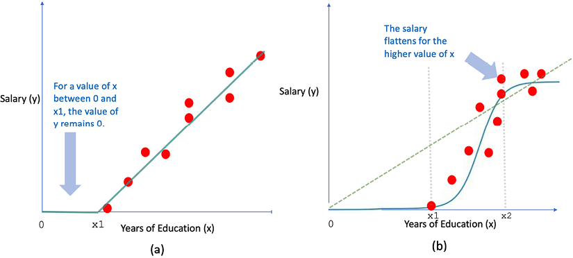
Figure 8.3: Salary and years of education

(a) Dataset 1: Linear patterns (b) Dataset 2: Non-linear patterns

Understanding layered deep learning architectures

For more complex problems, researchers have developed a multilayer neural network called a multilayer perceptron. A multilayer neural network has a few different layers, as shown in the following diagram. These layers are as follows:

• Input layer: The first layer is the input layer. At the input layer, the feature values are fed as input to the network.
• Hidden layer(s): The input layer is followed by one or more hidden layers. Each hidden layers are the arrays of similar activation functions.
• Output layer: The final layer is called the output layer.

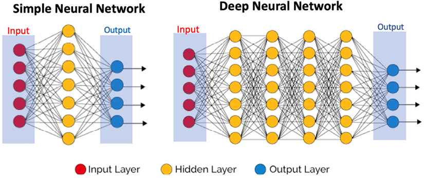
Figure 8.4: Simple neural network and deep neural network

Next, let us try to understand the function of hidden layers.

Developing an intuition for hidden layers

In a neural network, hidden layers play a key role in interpreting the input data. Hidden layers are methodically organized in a hierarchical structure within the neural network, where each layer performs a distinct non-linear transformation on its input data. This design allows for the extraction of progressively more abstract and nuanced features from the input.

Consider the example of convolutional neural networks, a subtype of neural networks specifically engineered for image-processing tasks. In this context, the lower hidden layers focus on discerning simple, local features such as edges and corners within an image. These features, while fundamental, don’t carry much meaning on their own.

As we move deeper into the hidden layers, these layers start to connect the dots, so to speak. They integrate the basic patterns detected by the lower layers, assembling them into more complex, meaningful structures. As a result, an originally incoherent scatter of edges and corners transforms into recognizable shapes and patterns, granting the network a level of “vision.”

This progressive transformation process turns unprocessed pixel values into an elaborate mapping of features and patterns, enabling advanced applications such as fingerprint recognition. Here, the network can pick out the unique arrangement of ridges and valleys in a fingerprint, converting this raw visual data into a unique identifier. Hence, hidden layers convert raw data and refined it into valuable insights.

How many hidden layers should be used?

Note that the optimal number of hidden layers will vary from problem to problem. For some problems, single-layer neural networks should be used. These problems typically exhibit straightforward patterns that can be easily captured and formulated by a minimalist network design. For others, we should add multiple layers for the best performance. For example, if you’re dealing with a complex problem, such as image recognition or natural language processing, a neural network with multiple hidden layers and a greater number of nodes in each layer might be necessary.

The complexity of your data’s underlying patterns will largely influence your network design. For instance, using an excessively complex neural network for a simple problem might lead to overfitting, where your model becomes too tailored to the training data and performs poorly on new, unseen data. On the other hand, a model that’s too simple for a complex problem might result in underfitting, where the model fails to capture essential patterns in the data.

Additionally, the choice of activation function plays a critical role. For example, if your output needs to be binary (like in a yes/no problem), a sigmoid function could be suitable. For multi-class classification problems, a softmax function might be better.

Ultimately, the process of selecting your neural network’s architecture requires careful analysis of your problem, coupled with experimentation and fine-tuning. This is where developing a baseline experimental model can be beneficial, allowing you to iteratively adjust and enhance your network’s design for optimal performance.

Let us next look into the mathematical basis of a neural network.

Mathematical basis of neural network

Understanding the mathematical foundation of neural networks is key to leveraging their power. While they may seem complex, the principles are based on familiar mathematical concepts such as linear algebra, calculus, and probability. The beauty of neural networks lies in their ability to learn from data and improve over time, attributes that are rooted in their mathematical structure:

Figure 8.5: A multi-layer perceptron

Figure 8.5 shows a 4-layer neural network. In this neural network, an important thing to note is that the neuron is the basic unit of this network, and each neuron of a layer is connected to all neurons of the next layer. For complex networks, the number of these interconnections explodes, and we will explore different ways of reducing these interconnections without sacrificing too much quality.

First, let’s try to formulate the problem we are trying to solve.

The input is a feature vector, x, of dimensions n.

We want the neural network to predict values. The predicted values are represented by ý.

Mathematically, we want to determine, given a particular input, the probability that a transaction is fraudulent. In other words, given a particular value of x, what is the probability that y = 1? Mathematically, we can represent this as follows:

Note that x is an n_x-dimensional vector, where n_x is the number of input variables.

The neural network shown in Figure 8.6 has four layers. The layers between the input and the output are the hidden layers. The number of neurons in the first hidden layer is denoted by . The links between various nodes are multiplied by parameters called weights. The process of training a neural network is fundamentally centered around determining the optimal values for the weights associated with the various connections between the network’s neurons. By adjusting these weights, the network can fine-tune its calculations and improve its performance over time.

Let’s see how we can train a neural network.

Training a neural network

The process of building a neural network using a given dataset is called training a neural network. Let’s look into the anatomy of a typical neural network. When we talk about training a neural network, we are talking about calculating the best values for the weights. The training is done iteratively by using a set of examples in the form of training data. The examples in the training data have the expected values of the output for different combinations of input values. The training process for neural networks is different from the way traditional models are trained (which was discussed in Chapter 7, Traditional Supervised Learning Algorithms).

Understanding the anatomy of a neural network

Let’s see what a neural network consists of:

• Layers: Layers are the core building blocks of a neural network. Each layer is a data-processing module that acts as a filter. It takes one or more inputs, processes them in a certain way, and then produces one or more outputs. Every time data passes through a layer, it goes through a processing phase and shows patterns that are relevant to the business question we are trying to answer.
• Loss function: The loss function provides the feedback signal that is used in the various iterations of the learning process. The loss function provides the deviation for a single example.
• Cost function: The cost function is the loss function on a complete set of examples.
• Optimizer: An optimizer determines how the feedback signal provided by the loss function will be interpreted.
• Input data: Input data is the data that is used to train the neural network. It specifies the target variable.
• Weights: The weights are calculated by training the network. Weights roughly correspond to the importance of each of the inputs. For example, if a particular input is more important than other inputs, after training, it is given a greater weight value, acting as a multiplier. Even a weak signal for that important input will gather strength from the large weight value (which acts as a multiplier). Thus weight ends up turning each of the inputs according to their importance.
• Activation function: The values are multiplied by different weights and then aggregated. Exactly how they will be aggregated and how their value will be interpreted will be determined by the type of the chosen activation function.

Let’s now have a look at a very important aspect of neural network training.

While training neural networks, we take each of the examples one by one. For each of the examples, we generate the output using our under-training model. The term “under-training” refers to the model’s learning state, where it is still adjusting and learning from data and has not reached its optimal performance yet. During this stage, the model parameters, such as weights, are constantly updated and adjusted to improve its predictive performance. We calculate the difference between the expected output and the predicted output. For each individual example, this difference is called the loss. Collectively, the loss across the complete training dataset is called the cost. As we keep on training the model, we aim to find the right values of weights that will result in the smallest loss value. Throughout the training, we keep on adjusting the values of the weights until we find the set of values for the weights that results in the minimum possible overall cost. Once we reach the minimum cost, we mark the model as trained.

Defining gradient descent

The central goal of training a neural network is to identify the correct values for the weights, which act like “dials” or “knobs” that we adjust to minimize the difference between the model’s predictions and the actual values.

When training begins, we initiate these weights with random or default values. We then progressively adjust them using an optimization algorithm, a popular choice being “gradient descent,” to incrementally improve our model’s predictions.

Let’s dive deeper into the gradient descent algorithm. The journey of gradient descent starts from the initial random values of weights that we set.

From this starting point, we iterate and, at each step, we adjust these weights to move us closer to the minimum cost.

To paint a clearer picture, imagine our data features as the input vector X. The true value of the target variable is Y, while the value our model predicts is Y. We measure the difference, or deviation, between these actual and predicted values. This difference gives us our loss.

We then update our weights, taking into account two key factors: the direction to move and the size of the step, also known as the learning rate.

The “direction” informs us where to move to find the minimum of the loss function. Think of this as descending a hill – we want to go “downhill” where the slope is steepest to get to the bottom (our minimum loss) the fastest.

The “learning rate” determines the size of our step in that chosen direction. It’s like deciding whether to walk or run down that hill – a larger learning rate means bigger steps (like running), and a smaller one means smaller steps (like walking).

The goal of this iterative process is to reach a point from which we can’t go “downhill”, meaning we have found the minimum cost, indicating our weights are now optimal, and our model is well trained.

This simple iterative process is shown in the following diagram:

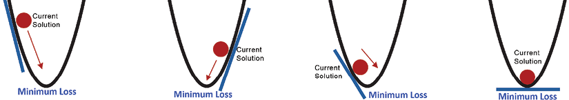
Figure 8.6: Gradient Descent Algorithm, finding the minimum

The diagram shows how, by varying the weights, gradient descent tries to find the minimum cost. The learning rate and chosen direction will determine the next point on the graph to explore.

Selecting the right value for the learning rate is important. If the learning rate is too small, the problem may take a lot of time to converge. If the learning rate is too high, the problem will not converge. In the preceding diagram, the dot representing our current solution will keep oscillating between the two opposite lines of the graph.

Now, let’s see how to minimize a gradient. Consider only two variables, x and y. The gradient of x and y is calculated as follows:

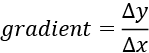
To minimize the gradient, the following approach can be used:

def adjust_position(gradient):
    while gradient != 0:
        if gradient < 0:
            print("Move right")
            # here would be your logic to move right
        elif gradient > 0:
            print("Move left")
            # here would be your logic to move left

This algorithm can also be used to find the optimal or near-optimal values of weights for a neural network.

Note that the calculation of gradient descent proceeds backward throughout the network. We start by calculating the gradient of the final layer first, and then the second-to-last one, and then the one before that, until we reach the first layer. This is called backpropagation, which was introduced by Hinton, Williams, and Rumelhart in 1985.

Next, let’s look into activation functions.

Activation functions

An activation function formulates how the inputs to a particular neuron will be processed to generate an output.

As shown in Figure 8.7, each of the neurons in a neural network has an activation function that determines how inputs will be processed:

Figure 8.7: Activation function

In the preceding diagram, we can see that the results generated by an activation function are passed on to the output. The activation function sets the criteria that how the values of the inputs are supposed to be interpreted to generate an output.

For exactly the same input values, different activation functions will produce different outputs. Understanding how to select the right activation function is important when using neural networks to solve problems.

Let’s now look into these activation functions one by one.

Step function

The simplest possible activation function is the threshold function. The output of the threshold function is binary: 0 or 1. It will generate 1 as the output if any of the inputs are greater than 1. This can be explained in Figure 8.8:

Figure 8.8: Step function

Despite its simplicity, the threshold activation function plays an important role, especially when we need a clear demarcation between the outputs. With this function, as soon as there’s any non-zero value in the weighted sums of inputs, the output (y) turns to 1. However, its simplicity has its drawbacks – the function is exceedingly sensitive and could be erroneously triggered by the slightest signal or noise in the input.

For instance, consider a situation where a neural network uses this function to classify emails into “spam” or “not spam.” Here, an output of 1 might represent “spam” and 0 might represent “not spam.” The slightest presence of a characteristic (like certain key spam words) could trigger the function to classify the email as “spam.” Hence, while it’s a valuable tool for certain use cases, its potential for over-sensitivity should be considered, especially in applications where noise or minor variances in input data are common. Next, let us look into the sigmoid function.

Sigmoid function

The sigmoid function can be thought of as an improvement of the threshold function. Here, we have control over the sensitivity of the activation function:

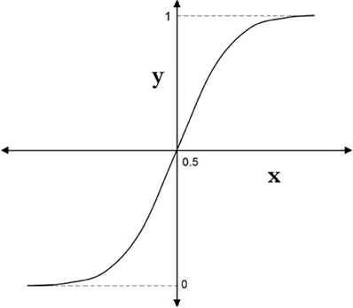
Figure 8.9: Sigmoid activation function

The sigmoid function, y, is defined as follows and shown in Figure 8.9:

It can be implemented in Python as follows:

def sigmoidFunction(z):
      return 1/ (1+np.exp(-z))

The code above demonstrates the sigmoid function using Python. Here, np.exp(-z) is the exponential operation applied to -z, and this term is added to 1 to form the denominator of the equation, resulting in a value between 0 and 1.

The reduction in the activation function’s sensitivity through the sigmoid function makes it less susceptible to sudden aberrations or “glitches” in the input. However, it’s worth noting that the output remains binary, meaning it can still only be 0 or 1.

Sigmoid functions are widely used in binary classification problems where the output is expected to be either 0 or 1. For instance, if you are developing a model to predict whether an email is spam (1) or not spam (0), a sigmoid activation function would be a suitable choice.

Now, let’s delve into the ReLU activation function.

ReLU

The output for the first two activation functions presented in this chapter was binary. That means that they will take a set of input variables and convert them into binary outputs. ReLU is an activation function that takes a set of input variables as input and converts them into a single continuous output. In neural networks, ReLU is the most popular activation function and is usually used in the hidden layers, where we do not want to convert continuous variables into category variables.

The following diagram summarizes the ReLU activation function:

Figure 8.10: ReLU

Note that when x ≤ 0, that means y = 0. This means that any signal from the input that is zero or less than zero is translated into a zero output:

As soon as x becomes more than zero, it is x.

The ReLU function is one of the most used activation functions in neural networks. It can be implemented in Python as follows:

def relu(x):
    if x < 0:
        return 0
    else:
        return x

Now let’s look into Leaky ReLU, which is based on ReLU.

Leaky ReLU

In ReLU, a negative value for x results in a zero value for y. This means that some information is lost in the process, which makes training cycles longer, especially at the start of training. The Leaky ReLU activation function resolves this issue. The following applies to Leaky ReLu:

This is shown in the following diagram:

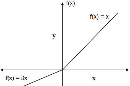
Figure 8.11: Leaky ReLU

Here, is a parameter with a value less than one.

It can be implemented in Python as follows:

def leaky_relu(x, beta=0.01):
    if x < 0:
        return beta * x    
    else:        
        return x

There are various strategies for assigning a value to :

• Default value: We can assign a default value to , typically 0.01. This is the most straightforward approach and can be useful in scenarios where we want a quick implementation without any intricate tuning.
• Parametric ReLU: Another approach is to allow to be a tunable parameter in our neural network model. In this case, the optimal value for is learned during the training process itself. This is beneficial in scenarios where we aim to tailor our activation function to the specific patterns present in our data.
• Randomized ReLU: We could also choose to randomly assign a value to . This technique, known as randomized ReLU, can act as a form of regularization and help prevent overfitting by introducing some randomness into the model. This could be helpful in scenarios where we have a large dataset with complex patterns and we want to ensure our model doesn’t overfit to the training data.

Hyperbolic tangent (tanh)

The hyperbolic tangent function, or tanh, is closely related to the sigmoid function, with a key distinction: it can output negative values, thereby offering a broader output range between -1 and 1. This can be useful in situations where we want to model phenomena that contain both positive and negative influences. Figure 8.12 illustrates this:

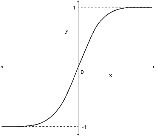
Figure 8.12: Hyperbolic tangent

The y function is as follows:

It can be implemented by the following Python code:

import numpy as np
def tanh(x): 
    numerator = 1 - np.exp(-2 * x) 
    denominator = 1 + np.exp(-2 * x) 
    return numerator / denominator

In this Python code, we’re using the numpy library, indicated by np, to handle the mathematical operations. The tanh function, like the sigmoid, is an activation function used in neural networks to add non-linearity to the model. It is often preferred over the sigmoid function in hidden layers of a neural network as it centers the data by making the output mean 0, which can make learning in the next layer easier. However, the choice between tanh, sigmoid, or any other activation function largely depends on the specific needs and complexities of the model you’re working with.

Moving on, let’s now delve into the softmax function.

Softmax

Sometimes, we need more than two levels for the output of the activation function. Softmax is an activation function that provides us with more than two levels for the output. It is best suited to multiclass classification problems. Let’s assume that we have n classes. We have input values. The input values map the classes as follows:

x = {x⁽¹⁾,x⁽²⁾,....x⁽ⁿ⁾}

Softmax operates on probability theory. For binary classifiers, the activation function in the final layer will be sigmoid, and for multiclass classifiers, it will be softmax. To illustrate, let’s say we’re trying to classify an image of a fruit, where the classes are apple, banana, cherry, and date. The softmax function calculates the probabilities of the image belonging to each of these classes. The class with the highest probability is then considered as the prediction.

To break this down in terms of Python code and equations, let’s look at the following:

import numpy as np
def softmax(x): 
    return np.exp(x) / np.sum(np.exp(x), axis=0)

In this code snippet, we’re using the numpy library (np) to perform the mathematical operations. The softmax function takes an array of x as input, applies the exponential function to each element, and normalizes the results so that they sum up to 1, which is the total probability across all classes.

Now let us look into various tools and frameworks related to neural networks.

Tools and frameworks

In this section, we will delve into the vast array of tools and frameworks that have been developed specifically to facilitate the implementation of neural networks. Each of these frameworks has its unique advantages and possible limitations.

Among the numerous options available, we’ve chosen to spotlight Keras, a high-level neural network API, which is capable of running on top of TensorFlow. Why Keras and TensorFlow, you may wonder? Well, these two in combination offer several notable benefits that make them a popular choice among practitioners.

Firstly, Keras, with its user-friendly and modular nature, simplifies the process of building and designing neural network models, thereby catering to beginners as well as experienced users. Secondly, its compatibility with TensorFlow, a powerful end-to-end open-source platform for ML, ensures robustness and versatility. TensorFlow’s ability to deliver high computational performance is another valuable asset. Together, they form a dynamic duo that strikes a balance between usability and functionality, making them an excellent choice for the development and deployment of neural network models.

In the following sections, we’ll explore more about how to use Keras with a TensorFlow backend to construct neural networks.

Keras

Keras (https://www.tensorflow.org/guide/keras) is one of the most popular and easy-to-use neural network libraries and is written in Python. It was written with ease of use in mind and provides the fastest way to implement deep learning. Keras only provides high-level blocks and is considered at the model level.

Now, let’s look into the various backend engines of Keras.

Backend engines of Keras

Keras needs a lower-level deep learning library to perform tensor-level manipulations. This foundational layer is referred to as the “backend engine.”

In simpler terms, tensor-level manipulations involve the computations and transformations that are performed on multi-dimensional arrays of data, known as tensors, which are the primary data structure used in neural networks. This lower-level deep-learning library is called the backend engine. Possible backend engines for Keras include the following:

• TensorFlow (www.tensorflow.org): This is the most popular framework of its kind and is open sourced by Google.
• Theano: This was developed at the MILA lab at Université de Montréal.
• Microsoft Cognitive Toolkit (CNTK) (https://learn.microsoft.com/en-us/cognitive-toolkit/): This was developed by Microsoft.

The format of this modular deep learning technology stack is shown in the following diagram:

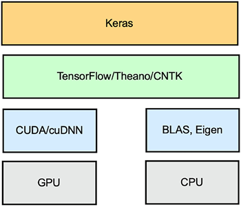
Figure 8.13: Keras architecture

The advantage of this modular deep learning architecture is that the backend of Keras can be changed without rewriting any code. For example, if we find TensorFlow better than Theona for a particular task, we can simply change the backend to TensorFlow without rewriting any code.

Next, let us look into the low-level layers of the deep learning stack.

Low-level layers of the deep learning stack

The three backend engines we just mentioned can all run both on CPUs and GPUs using the low-level layers of the stack. For CPUs, a low-level library of tensor operations called Eigen is used. For GPUs, TensorFlow uses NVIDIA’s CUDA Deep Neural Network (cuDNN) library. It’s noteworthy to explain why GPUs are often preferred in ML.

While CPUs are versatile and capable, GPUs are specifically designed to handle multiple operations concurrently, which is beneficial when processing large blocks of data, a common occurrence in ML tasks. This trait of GPUs, combined with their higher memory bandwidth, can significantly expedite ML computations, thereby making them a popular choice for such tasks.

Next, let us explain the hyperparameters.

Defining hyperparameters

As discussed in Chapter 6, Unsupervised Machine Learning Algorithms, a hyperparameter is a parameter whose value is chosen before the learning process starts. We start with common-sense values and then try to optimize them later. For neural networks, the important hyperparameters are these:

• The activation function
• The learning rate
• The number of hidden layers
• The number of neurons in each hidden layer

Let’s look into how we can define a model using Keras.

Defining a Keras model

There are three steps involved in defining a complete Keras model:

1. Define the layers
2. Define the learning process
3. Test the model

We can build a model using Keras in two possible ways:

• The Functional API: This allows us to architect models for acyclic graphs of layers. More complex models can be created using the Functional API.
• The Sequential API: This allows us to architect models for a linear stack of layers. It is used for relatively simple models and is the usual choice for building models.

First, we take a look at the Sequential way of defining a Keras model:

1. Let us start with importing the tensorflow library:

   import tensorflow as tf
   
2. Then, load the MNIST dataset from Keras’ datasets:

   mnist = tf.keras.datasets.mnist
   
3. Next, split the dataset into training and test sets:

   (train_images, train_labels), (test_images, test_labels) = mnist.load_data()
   
4. We normalize the pixel values from a scale out of 255 to a scale out of 1:

   train_images, test_images = train_images / 255.0,                             test_images / 255.0
   
5. Next, we define the structure of the model:

   model = tf.keras.models.Sequential([
       tf.keras.layers.Flatten(input_shape=(28, 28)),
       tf.keras.layers.Dense(128, activation='relu'),
       tf.keras.layers.Dropout(0.15),
       tf.keras.layers.Dense(128, activation='relu'),
       tf.keras.layers.Dropout(0.15),
       tf.keras.layers.Dense(10, activation='softmax'),
   ])
   

This script is training a model to classify images from the MNIST dataset, which is a set of 70,000 small images of digits handwritten by high school students and employees of the US Census Bureau.

The model is defined using the Sequential method in Keras, indicating that our model is organized as a linear stack of layers:

1. The first layer is a Flatten layer, which transforms the format of the images from a two-dimensional array into a one-dimensional array.
2. The next layer, a Dense layer, is a fully connected neural layer with 128 nodes (or neurons). The relu (ReLU) activation function is used here.
3. The Dropout layer randomly sets input units to 0 with a frequency of rate at each step during training time, which helps prevent overfitting.
4. Another Dense layer is included; similar to the previous one, it’s also using the relu activation function.
5. We again apply a Dropout layer with the same rate as before.
6. The final layer is a 10-node softmax layer—this returns an array of 10 probability scores that sums to 1. Each node contains a score that indicates the probability that the current image belongs to one of the 10 digit classes.

Note that, here, we have created three layers – the first two layers have the relu activation function and the third layer has softmax as the activation function.

Now, let’s take a look at the Functional API way of defining a Keras model:

1. First, let us import the tensorflow library:

   # Ensure TensorFlow 2.x is being used
   %tensorflow_version 2.x
   import tensorflow as tf
   from tensorflow.keras.datasets import mnist
   
2. To work with the MNIST dataset, we first load it into memory. The dataset is conveniently split into training and testing sets, with both images and corresponding labels:

   # Load MNIST dataset
   (train_images, train_labels), (test_images, test_labels) = mnist.load_data()
   # Normalize the pixel values to be between 0 and 1
   train_images, test_images = train_images / 255.0, test_images / 255.0
   
3. The images in the MNIST dataset are 28x28 pixels in size. When setting up a neural network model using TensorFlow, you need to specify the shape of the input data, Here, we establish the input tensor for the model:

   inputs = tf.keras.Input(shape=(28,28))
   
4. Next, the Flatten layer is a simple data preprocessing step. It transforms the two-dimensional 128x128 pixel input into a one-dimensional array by “flattening” it. This prepares the data for the following Dense layer:

   x = tf.keras.layers.Flatten()(inputs)
   
5. Then comes the first Dense layer, also known as a fully connected layer, in which each input node (or neuron) is connected to each output node. The layer has 512 output nodes and uses the relu activation function. ReLU is a popular choice of activation function that outputs the input directly if it is positive; otherwise, it outputs zero:

   x = tf.keras.layers.Dense(512, activation='relu', name='d1')(x)
   
6. The Dropout layer randomly sets a fraction (0.2, or 20% in this case) of the input nodes to 0 at each update during training, which helps prevent overfitting:

   x = tf.keras.layers.Dropout(0.2)(x)
   
7. Finally, comes the output layer. It’s another Dense layer with 10 output nodes (presumably for 10 classes). The softmax activation function is applied, which outputs a probability distribution over the 10 classes, meaning it will output 10 values that sum to 1. Each value represents the model’s confidence that the input image corresponds to a particular class:

   predictions = tf.keras.layers.Dense(10, activation=tf.nn.softmax, name='d2')(x)
   model = tf.keras.Model(inputs=inputs, outputs=predictions)
   

Note that we can define the same neural network using both the Sequential and Functional APIs. From the point of view of performance, it does not make any difference which approach you take to define the model.

Let us convert the numerical train_labels and test_labels into one-hot encoded vectors. In the following code each label becomes a binary array of size 10 with a 1 at its respective digit’s index and 0s elsewhere:

# One-hot encode the labels
train_labels_one_hot = tf.keras.utils.to_categorical(train_labels, 10)
test_labels_one_hot = tf.keras.utils.to_categorical(test_labels, 10)

We should now define the learning process.

In this step, we define three things:

• The optimizer
• The loss function
• The metrics that will quantify the quality of the model:

optimizer = tf.keras.optimizers.RMSprop()
loss = 'categorical_crossentropy'
metrics = ['accuracy']
model.compile(optimizer=optimizer, loss=loss, metrics=metrics)

Note that we use the model.compile function to define the optimizer, loss function, and metrics.

We will now train the model.

Once the architecture is defined, it is time to train the model:

history = model.fit(train_images, train_labels_one_hot, epochs=10, validation_data=(test_images, test_labels_one_hot))

Note that parameters such as batch_size and epochs are configurable parameters, making them hyperparameters.

Next, let us look into how we can choose the sequential or functional model.

Choosing a sequential or functional model

When deciding between using a sequential or functional model to construct a neural network, the nature of your network’s architecture will guide your choice. The sequential model is suited to simple linear stacks of layers. It’s uncomplicated and straightforward to implement, making it an ideal choice for beginners or for simpler tasks. However, this model comes with a key limitation: each layer can be connected to precisely one input tensor and one output tensor.

If the architecture of your network is more complex, such as having multiple inputs or outputs at any stage (input, output, or hidden layers), then the sequential model falls short. For such complex architectures, the functional model is more appropriate. This model provides a higher degree of flexibility, allowing for more complex network structures with multiple inputs and outputs at any layer. Let us now develop a deeper understanding of TensorFlow.

Understanding TensorFlow

TensorFlow is one of the most popular libraries for working with neural networks. In the preceding section, we saw how we can use it as the backend engine of Keras. It is an open-source, high-performance library that can actually be used for any numerical computation.

If we look at the stack, we can see that we can write TensorFlow code in a high-level language such as Python or C++, which gets interpreted by the TensorFlow distributed execution engine. This makes it quite useful for and popular with developers.

TensorFlow functions by using a directed graph (DG) to embody your computations. In this graph, nodes are mathematical operations, and the edges connecting these nodes signify the input and output of these operations. Moreover, these edges symbolize data arrays.

Apart from serving as the backend engine for Keras, TensorFlow is broadly used in various scenarios. It can help in developing complex ML models, processing large datasets, and even deploying AI applications across different platforms. Whether you’re creating a recommendation system, image classification model, or natural language processing tool, TensorFlow can effectively cater to these tasks and more.

Presenting TensorFlow’s basic concepts

Let’s take a brief look at TensorFlow concepts such as scalars, vectors, and matrices. We know that a simple number, such as three or five, is called a scalar in traditional mathematics. Moreover, in physics, a vector is something with magnitude and direction. In terms of TensorFlow, we use a vector to mean one-dimensional arrays. Extending this concept, a two-dimensional array is a matrix. For a three-dimensional array, we use the term 3D tensor. We use the term rank to capture the dimensionality of a data structure. As such, a scalar is a rank 0 data structure, a vector is a rank 1 data structure, and a matrix is a rank 2 data structure. These multi-dimensional structures are known as tensors and are shown in the following diagram:

Figure 8.14: Multi-dimensional structures or tensors

As we can see in the preceding diagram, the rank defines the dimensionality of a tensor.

Let’s now look at another parameter, shape. shape is a tuple of integers specifying the length of an array in each dimension.

The following diagram explains the concept of shape:

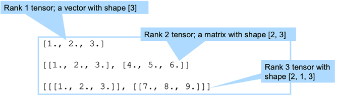
Figure 8.15: Concept of a shape

Using shape and ranks, we can specify the details of tensors.

Understanding Tensor mathematics

Let’s now look at different mathematical computations using tensors:

• Let’s define two scalars and try to add and multiply them using TensorFlow:

  print("Define constant tensors")
  a = tf.constant(2)
  print("a = %i" % a)
  b = tf.constant(3)
  print("b = %i" % b)
  

  Define constant tensors
  a = 2
  b = 3
  
• We can add and multiply them and display the results:

  print("Running operations, without tf.Session")
  c = a + b
  print("a + b = %i" % c)
  d = a * b
  print("a * b = %i" % d)
  

  Running operations, without tf.Session
  a + b = 5
  a * b = 6
  
• We can also create a new scalar tensor by adding the two tensors:

  c = a + b
  print("a + b = %s" % c)
  

  a + b = tf.Tensor(5, shape=(), dtype=int32)
  
• We can also perform complex tensor functions:

  d = a*b
  print("a * b = %s" % d)
  

  a * b = tf.Tensor(6, shape=(), dtype=int32)
  

Understanding the types of neural networks

Neural networks can be designed in various ways, depending on how the neurons are interconnected. In a dense, or fully connected, neural network, every single neuron in a given layer is linked to each neuron in the next layer. This means each input from the preceding layer is fed into every neuron of the subsequent layer, maximizing the flow of information.

However, neural networks aren’t always fully connected. Some may have specific patterns of connections based on the problem they are designed to solve. For instance, in convolutional neural networks used for image processing, each neuron in a layer may only be connected to a small region of neurons in the previous layer. This mirrors the way neurons in the human visual cortex are organized and helps the network efficiently process visual information.

Remember, the specific architecture of a neural network – how the neurons are interconnected – greatly impacts its functionality and performance.

Convolutional neural networks

Convolution neural networks (CNNs) are typically used to analyze multimedia data. In order to learn more about how a CNN is used to analyze image-based data, we need to have a grasp of the following processes:

• Convolution
• Pooling

Let’s explore them one by one.

Convolution

The process of convolution emphasizes a pattern of interest in a particular image by processing it with another smaller image called a filter (also called a kernel). For example, if we want to find the edges of objects in an image, we can convolve the image with a particular filter to get them. Edge detection can help us in object detection, object classification, and other applications. So, the process of convolution is about finding characteristics and features in an image.

The approach to finding patterns is based on finding patterns that can be reused on different data. The reusable patterns are called filters or kernels.

Pooling

An important part of processing multimedia data for the purpose of ML is downsampling it. Downsampling is the practice of reducing the resolution of your data, i.e., lessening the data’s complexity or dimensionality. Pooling offers two key advantages:

• By reducing the data’s complexity, we significantly decrease the training time for the model, enhancing computational efficiency.
• Pooling abstracts and aggregates unnecessary details in the multimedia data, making it more generalized. This, in turn, enhances the model’s ability to represent similar problems.

Downsampling is performed as follows:

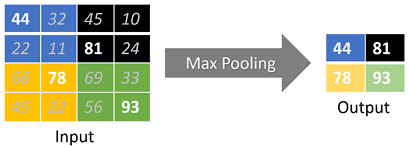
Figure 8.16: Downsampling

In the downsampling process, we essentially condense a group of pixels into a single representative pixel. For instance, let’s say we condense a 2x2-pixel block into a single pixel, effectively downsampling the original data by a factor of four.

The representative value for the new pixel can be chosen in various ways. One such method is “max pooling,” where we select the maximum value from the original pixel block to represent the new single pixel.

On the other hand, if we chose to take the average of the pixel block’s values, the process would be termed “average pooling.”

The choice between max pooling and average pooling often depends on the specific task at hand. Max pooling is particularly beneficial when we’re interested in preserving the most prominent features of the image, as it retains the maximum pixel value in a block, thus capturing the most standout or noticeable aspect within that section.

In contrast, average pooling tends to be useful when we want to preserve the overall context and reduce noise, as it considers all values within a block and calculates their average, creating a more balanced representation that may be less sensitive to minor variations or noise in pixel values.

Generative Adversarial Networks

Generative Adversarial Networks, commonly referred to as GANs, represent a distinct class of neural networks capable of generating synthetic data. First introduced by Ian Goodfellow and his team in 2014, GANs have been hailed for their innovative approach to creating new data resembling the original training samples.

One notable application of GANs is their ability to produce realistic images of people who don’t exist in reality, showcasing their remarkable capacity for detail generation. However, an even more crucial application lies in their potential to generate synthetic data, thereby augmenting existing training datasets, which can be extremely beneficial in scenarios where data availability is limited.

Despite their potential, GANs are not without limitations. The training process of GANs can be quite challenging, often leading to issues such as mode collapse, where the generator starts producing limited varieties of samples. Additionally, the quality of the generated data is largely dependent on the quality and diversity of the input data. Poorly representative or biased data can result in less effective, potentially skewed synthetic data.

In the upcoming section, we will see what transfer learning is.

Using transfer learning

Throughout the years, countless organizations, research entities, and contributors within the open-source community have meticulously built sophisticated models for general use cases. These models, often trained with vast amounts of data, have been optimized over years of hard work and are suited for various applications, such as:

• Detecting objects in videos or images
• Transcribing audio
• Analyzing sentiment in text

When initiating the training of a new ML model, it’s worth questioning, rather than starting from a blank slate, whether we can modify an already established, pre-trained model to suit our needs. Put simply, could we leverage the learning of existing models to tailor a custom model that addresses our specific needs? Such an approach, known as transfer learning, can provide several advantages:

• It gives a head start to our model training.
• It potentially enhances the quality of our model by utilizing a pre-validated and reliable model.
• In cases where our problem lacks sufficient data, transfer learning using a pre-trained model can be of immense help.

Consider the following practical examples where transfer learning would be beneficial:

• For training a robot, a neural network model could first be trained using a simulation game. In this controlled environment, we can create rare events that are difficult to replicate in the real world. Once trained, transfer learning can then be applied to adapt the model for real-world scenarios.
• Suppose we aim to build a model that distinguishes between Apple and Windows laptops in a video feed. Existing, open-source object detection models, known for their accuracy in classifying diverse objects in video feeds, could serve as an ideal starting point. Using transfer learning, we can first leverage these models to identify objects as laptops. Subsequently, we could refine our model further to differentiate between Apple and Windows laptops.

In our next section, we will implement the principles discussed in this chapter to create a neural network for classifying fraudulent documents.

As a visual example, consider a pre-trained model as a well-established tree with many branches (layers). Some branches are already ripe with fruits (trained to identify features). When applying transfer learning, we “freeze” these fruitful branches, preserving their established learning. We then allow new branches to grow and bear fruit, which is akin to training the additional layers to understand our specific features. This process of freezing some layers and training others encapsulates the essence of transfer learning.

Case study – using deep learning for fraud detection

Using ML techniques to identify fraudulent documents is an active and challenging field of research. Researchers are investigating to what extent the pattern recognition power of neural networks can be exploited for this purpose. Instead of manual attribute extractors, raw pixels can be used for several deep learning architectural structures.

Methodology

The technique presented in this section uses a type of neural network architecture called Siamese neural networks, which features two branches that share identical architectures and parameters.

The use of Siamese neural networks to flag fraudulent documents is shown in the following diagram:

Figure 8.17: Siamese neural networks

When a particular document needs to be verified for authenticity, we first classify the document based on its layout and type, and then we compare it against its expected template and pattern. If it deviates beyond a certain threshold, it is flagged as a fake document; otherwise, it is considered an authentic or true document. For critical use cases, we can add a manual process for borderline cases where the algorithm conclusively classifies a document as authentic or fake.

To compare a document against its expected template, we use two identical CNNs in our Siamese architecture. CNNs have the advantage of learning optimal shift-invariant local feature detectors and can build representations that are robust to geometric distortions of the input image. This is well suited to our problem since we aim to pass authentic and test documents through a single network, and then compare their outcomes for similarity. To achieve this goal, we implement the following steps.

Let’s assume that we want to test a document. For each class of document, we perform the following steps:

1. Get the stored image of the authentic document. We call it the true document. The test document should look like the true document.
2. The true document is passed through the neural network layers to create a feature vector, which is the mathematical representation of the patterns of the true document. We call it Feature Vector 1, as shown in the preceding diagram.
3. The document that needs to be tested is called the test document. We pass this document through a neural network similar to the one that was used to create the feature vector for the true document. The feature vector of the test document is called Feature Vector 2.
4. We use the Euclidean distance between Feature Vector 1 and Feature Vector 2 to calculate the similarity score between the true document and the test document. This similarity score is called the Measure Of Similarity (MOS). The MOS is a number between 0 and 1. A higher number represents a lower distance between the documents and a greater likelihood that the documents are similar.
5. If the similarity score calculated by the neural network is below a pre-defined threshold, we flag the document as fraudulent.

Let’s see how we can implement Siamese neural networks using Python.

To illustrate how we can implement Siamese neural networks using Python, we’ll break down the process into simpler, more manageable blocks. This approach will help us follow the PEP8 style guide and keep our code readable and maintainable:

1. First, let’s import the Python packages that are required:

   import random
   import numpy as np
   import tensorflow as tf
   
2. Next, we define the network model that will process each branch of the Siamese network. Note that we’ve incorporated a dropout rate of 0.15 to mitigate overfitting:

   def createTemplate():
       return tf.keras.models.Sequential([
           tf.keras.layers.Flatten(),
           tf.keras.layers.Dense(128, activation='relu'),
           tf.keras.layers.Dropout(0.15),
           tf.keras.layers.Dense(128, activation='relu'),
           tf.keras.layers.Dropout(0.15),
           tf.keras.layers.Dense(64, activation='relu'), 
       ])
   
3. For our Siamese networks, we’ll use MNIST images. These images are excellent for testing the effectiveness of our Siamese network. We prepare the data such that each sample will contain two images and a binary similarity flag indicating whether they belong to the same class:

   def prepareData(inputs: np.ndarray, labels: np.ndarray):
       classesNumbers = 10
       digitalIdx = [np.where(labels == i)[0] for i in range(classesNumbers)]
   
4. In the prepareData function, we ensure an equal number of samples across all digits. We first create an index of where in our dataset each digit appears, using the np.where function.

   Then, we prepare our pairs of images and assign labels:

       pairs = list()
       labels = list()
       n = min([len(digitalIdx[d]) for d in range(classesNumbers)]) - 1
       for d in range(classesNumbers):
           for i in range(n):
               z1, z2 = digitalIdx[d][i], digitalIdx[d][i + 1]
               pairs += [[inputs[z1], inputs[z2]]]
               inc = random.randrange(1, classesNumbers)
               dn = (d + inc) % classesNumbers
               z1, z2 = digitalIdx[d][i], digitalIdx[dn][i]
               pairs += [[inputs[z1], inputs[z2]]]
               labels += [1, 0] 
       return np.array(pairs), np.array(labels, dtype=np.float32)
   

5. Subsequently, we’ll prepare our training and testing datasets:

   input_a = tf.keras.layers.Input(shape=input_shape)
   encoder1 = base_network(input_a)
   input_b = tf.keras.layers.Input(shape=input_shape)
   encoder2 = base_network(input_b)
   
6. Lastly, we will implement the MOS, which quantifies the distance between two documents that we want to compare:

   distance = tf.keras.layers.Lambda( 
       lambda embeddings: tf.keras.backend.abs(
           embeddings[0] - embeddings[1]
       )
   ) ([encoder1, encoder2])
   measureOfSimilarity = tf.keras.layers.Dense(1, activation='sigmoid') (distance)
   

Now, let’s train the model. We will use 10 epochs to train this model:

# Build the model
model = tf.keras.models.Model([input_a, input_b], measureOfSimilarity)
# Train
model.compile(loss='binary_crossentropy',optimizer=tf.keras.optimizers.Adam(),metrics=['accuracy'])
model.fit([train_pairs[:, 0], train_pairs[:, 1]], tr_labels, 
          batch_size=128,epochs=10,validation_data=([test_pairs[:, 0], test_pairs[:, 1]], test_labels))

Epoch 1/10
847/847 [==============================] - 6s 7ms/step - loss: 0.3459 - accuracy: 0.8500 - val_loss: 0.2652 - val_accuracy: 0.9105
Epoch 2/10
847/847 [==============================] - 6s 7ms/step - loss: 0.1773 - accuracy: 0.9337 - val_loss: 0.1685 - val_accuracy: 0.9508
Epoch 3/10
847/847 [==============================] - 6s 7ms/step - loss: 0.1215 - accuracy: 0.9563 - val_loss: 0.1301 - val_accuracy: 0.9610
Epoch 4/10
847/847 [==============================] - 6s 7ms/step - loss: 0.0956 - accuracy: 0.9665 - val_loss: 0.1087 - val_accuracy: 0.9685
Epoch 5/10
847/847 [==============================] - 6s 7ms/step - loss: 0.0790 - accuracy: 0.9724 - val_loss: 0.1104 - val_accuracy: 0.9669
Epoch 6/10
847/847 [==============================] - 6s 7ms/step - loss: 0.0649 - accuracy: 0.9770 - val_loss: 0.0949 - val_accuracy: 0.9715
Epoch 7/10
847/847 [==============================] - 6s 7ms/step - loss: 0.0568 - accuracy: 0.9803 - val_loss: 0.0895 - val_accuracy: 0.9722
Epoch 8/10
847/847 [==============================] - 6s 7ms/step - loss: 0.0513 - accuracy: 0.9823 - val_loss: 0.0807 - val_accuracy: 0.9770
Epoch 9/10
847/847 [==============================] - 6s 7ms/step - loss: 0.0439 - accuracy: 0.9847 - val_loss: 0.0916 - val_accuracy: 0.9737
Epoch 10/10
847/847 [==============================] - 6s 7ms/step - loss: 0.0417 - accuracy: 0.9853 - val_loss: 0.0835 - val_accuracy: 0.9749
<tensorflow.python.keras.callbacks.History at 0x7ff1218297b8>

Note that we reached an accuracy of 97.49% using 10 epochs. Increasing the number of epochs will further improve the level of accuracy.

Summary

In this chapter, we journeyed through the evolution of neural networks, examining different types, key components like activation functions, and the significant gradient descent algorithm. We touched upon the concept of transfer learning and its practical application in identifying fraudulent documents.

As we proceed to the next chapter, we’ll delve into natural language processing, exploring areas such as word embedding and recurrent networks. We will also learn how to implement sentiment analysis. The captivating realm of neural networks continues to unfold.

Learn more on Discord

To join the Discord community for this book – where you can share feedback, ask questions to the author, and learn about new releases – follow the QR code below:

https://packt.link/WHLel