7

Traditional Supervised Learning Algorithms

Artificial intelligence is the new electricity.

—Andrew Ng

In Chapter 7, we will turn our attention to supervised machine learning algorithms. These algorithms, characterized by their reliance on labeled data for model training, are multifaceted and versatile in nature. Let’s consider some instances such as decision trees, Support Vector Machines (SVMs), and linear regression, to name a few, which all fall under the umbrella of supervised learning.

As we delve deeper into this field, it’s important to note that this chapter doesn’t cover neural networks, a significant category within supervised machine learning. Given their complexity and the rapid advancements occurring in the field, neural networks merit an in-depth exploration, which we will embark on in the following three chapters. The vast expanse of neural networks necessitates more than a single chapter to fully discuss their complexities and potential.

In this chapter, we will delve into the essentials of supervised machine learning, featuring classifiers and regressors. We will explore their capabilities using real-world problems as case studies. Six distinct classification algorithms will be presented, followed by three regression techniques. Lastly, we’ll compare their results to encapsulate the key takeaways from this discussion.

The overall objective of this chapter is for you to understand the different types of supervised machine learning techniques, and to know what the best supervised machine learning techniques are for certain classes of problems.

The following concepts are discussed in this chapter:

• Understanding supervised machine learning
• Understanding classification algorithms
• The methods to evaluate the performance of classifiers
• Understanding regression algorithms
• The methods to evaluate the performance of regression algorithms

Let’s start by looking at the basic concepts behind supervised machine learning.

Understanding supervised machine learning

Machine learning focuses on using data-driven approaches to create autonomous systems that can help us to make decisions with or without human supervision. In order to create these autonomous systems, machine learning uses a group of algorithms and methodologies to discover and formulate repeatable patterns in data. One of the most popular and powerful methodologies used in machine learning is the supervised machine learning approach. In supervised machine learning, an algorithm is given a set of inputs, called features, and their corresponding outputs, called labels. These features often comprise structured data like user profiles, historical sales figures, or sensor measurements, while the labels usually represent specific outcomes we want to predict, such as customer purchasing habits or product quality ratings. Using a given dataset, a supervised machine learning algorithm is used to train a model that captures the complex relationship between the features and labels represented by a mathematical formula. This trained model is the basic vehicle that is used for predictions.

Let’s consider an example where we want to use supervised machine learning techniques to train a model that can categorize a set of emails into legitimate ones (called legit) and unwanted ones (called spam). In order to get started, we need examples from the past so that the machine can learn what sort of content of emails should be classified as spam.

This content-based learning task using text data is a complex process and is achieved through one of the supervised machine learning algorithms. Some examples of supervised machine learning algorithms that can be used to train the model in this example include decision trees and Naive Bayes classifiers, which we will discuss later in this chapter.

For now, we will focus on how we can formulate supervised machine learning problems.

Formulating supervised machine learning problems

Before going deeper into the details of supervised machine learning algorithms, let’s define some of the basic supervised machine learning terminology:

A trained supervised machine learning model is capable of making predictions by estimating the label based on the features.

Let’s introduce the notation that we will use in this chapter to discuss the machine learning techniques:

Note that in this context, an “example” refers to a single instance in our dataset. Each example comprises a set of features (input data) and a corresponding label (the outcome we’re predicting)

Let’s delve into some practical applications of the terms we’ve introduced. Consider a feature vector, essentially a data structure encompassing all the features.

For instance, if we have “n” features and “b” training examples, we represent this training feature vector as X_train. Hence, if our training dataset consists of five examples and five variables or features, X_train will have five rows—one for each example, and a total of 25 elements (5 examples x 5 features).

In this context, X_train is a specific term representing our training dataset. Each example in this dataset is a combination of features and its associated label. We use superscripts to denote a specific example’s row number. Thus, a single example in our dataset is given as (X⁽¹⁾, y⁽¹⁾) where X⁽¹⁾ refers to the features of the first example and y⁽¹⁾ is its corresponding label.

Our complete labeled dataset, D, can therefore be expressed as D = {( X⁽¹⁾,y⁽¹⁾), (y ⁽²⁾,y⁽²⁾), ….. , (X^(d),y^(d))}, where D signifies the total number of examples.

We partition D into two subsets - the training set D_train and the testing set D_test. The training set, D_train, can be depicted as D_train = {( X⁽¹⁾,y⁽¹⁾), (X⁽²⁾,y⁽²⁾), ….. , (X^(b),y^(b))}, where ‘b’ is the number of training examples.

The primary goal of training a model is to ensure that the predicted target value ('ý') for any i^th example in the training set aligns as closely as possible with the actual label ('y'). This ensures that the model’s predictions reflect the true outcomes presented in the examples.

Now, let’s see how some of these terminologies are formulated practically.

As we discussed, a feature vector is defined as a data structure that has all the features stored in it.

If the number of features is n and the number of training examples is b, then X_train represents the training feature vector.

For the training dataset, the feature vector is represented by X_train. If there are b examples in the training dataset, then X_train will have b rows. If there are n variables, then the training dataset will have a dimension of n x b.

We will use superscript to represent the row number of a training example.

This particular example in our labeled dataset is represented by (Features⁽¹⁾,label⁽¹⁾) = (X⁽¹⁾, y⁽¹⁾).

So, our labeled dataset is represented by D = {(X⁽¹⁾,y⁽¹⁾), (X⁽²⁾,y⁽²⁾), ….. , (X^(d),y^(d))}.

We divide that into two parts—D_train and D_test.

So, our training set can be represented by D_train = {(X⁽¹⁾,y⁽¹⁾), (X⁽²⁾,y⁽²⁾), ….. , (X^(b),y^(b))}.

The objective of training a model is that for any i^th example in the training set, the predicted value of the target value should be as close to the actual value in the examples as possible. In other words:

So, our testing set can be represented by D_test = {X⁽¹⁾,y⁽¹⁾), (X⁽²⁾,y⁽²⁾), ..... , (X^(c),y^(c))}.

The values of the label are represented by a vector, Y:

Y ={y⁽¹⁾, y⁽²⁾, ....., y^(m)}

Let’s illustrate the concepts with an example.

Let’s imagine we’re working on a project to predict house prices based on various features, like the number of bedrooms, the size of the house in square feet, and its age. Here’s how we’d apply our machine learning terminology to this real-world scenario.

In this context, our “features” would be the number of bedrooms, house size, and age. Let’s say we have 50 examples (i.e., 50 different houses for which we have these details and the corresponding price). We can represent these in a training feature vector called X_train.

X_train becomes a table with 50 rows (one for each house) and 3 columns (one for each feature: bedrooms, size, and age). It’s a 50 x 3 matrix holding all our feature data.

An individual house’s feature set and price might be represented as ((X⁽ⁱ⁾,y⁽ⁱ⁾)), where X⁽ⁱ⁾ contains the features of the i^th house and y⁽ⁱ⁾ is its actual price.

Our entire dataset D can then be viewed as D = {(X⁽¹⁾,y⁽¹⁾), (X⁽²⁾,y⁽²⁾)), ... , ((X⁽⁵⁰⁾,y⁽⁵⁰⁾))}.

Suppose we use 40 houses for training and the remaining 10 for testing. Our training set D_train would be the first 40 examples: {(X⁽¹⁾,y⁽¹⁾), (X⁽²⁾,y⁽²⁾)), ... , ((X⁽⁴⁰⁾,y⁽⁴⁰⁾))}.

After training our model, the goal is to predict house prices that closely match the actual prices for all houses in our training set.

Our testing set D_test consists of the remaining 10 examples: {(X⁽⁴¹⁾,y⁽⁴¹⁾), (X⁽⁴²⁾,y⁽⁴²⁾), ... , (X⁽⁵⁰⁾,y⁽⁵⁰⁾))}.

Lastly, we have the Y vector, comprising all our actual house prices: Y ={ y⁽¹⁾, y⁽²⁾, ....., y⁽⁵⁰⁾}.

With this concrete example, we can see how these concepts and equations translate into practice when predicting house prices with supervised machine learning.

Understanding enabling conditions

A supervised machine learning algorithm needs certain enabling conditions to be met in order to perform. Enabling conditions are certain prerequisites that ensure the efficacy of a supervised machine learning algorithm. These enabling conditions are as follows:

• Enough examples: Supervised machine learning algorithms need enough examples to train a model. We say that we have enough examples when we have conclusive evidence that the pattern of interest is fully represented in our dataset.
• Patterns in historical data: The examples used to train a model need to have patterns in them. The likelihood of the occurrence of our event of interest should be dependent on a combination of patterns, trends, and events. The label mathematically represents the event of interest in our model. Without these, we are dealing with random data that cannot be used to train a model.
• Valid assumptions: When we train a supervised machine learning model using examples, we expect that the assumptions that apply to the examples will also be valid in the future. Let’s look at an actual example. If we want to train a machine learning model for the government that can predict the likelihood of whether a visa will be granted to a student, the understanding is that the laws and policies will not change when the model is used for predictions. If new policies or laws are enforced after training the model, the model may need to be retrained to incorporate this new information.

Let us look into how we can differentiate between a classifier and a regressor.

Differentiating between classifiers and regressors

In a machine learning model, the label can be a category variable or a continuous variable. Continuous variables are numeric variables that can have an infinite number of values between two values, while categorical variables are qualitative variables that are classified into distinct categories. The type of label determines what type of supervised machine learning model we have. Fundamentally, we have two types of supervised machine learning models:

• Classifiers: If the label is a category variable, the machine learning model is called a classifier. Classifiers can be used to answer the following type of business questions:
  • Is this abnormal tissue growth a malignant tumor?
  • Based on the current weather conditions, will it rain tomorrow?
  • Based on the profile of a particular applicant, should their mortgage application be approved?
• Regressors: If the label is a continuous variable, we train a regressor. Regressors can be used to answer the following types of business questions:
  • Based on the current weather condition, how much will it rain tomorrow?
  • What will the price of a particular home be with given characteristics?

Let’s look at both classifiers and regressors in more detail.

Understanding classification algorithms

In supervised machine learning, if the label is a category variable, the model is categorized as a classifier. Recall that the model is essentially a mathematical representation learned from the training data:

• The historical data is called labeled data.
• The production data, which the label needs to be predicted for, is called unlabeled data.

Before we present the details of classification algorithms, let’s first present a business problem that we will use as a challenge for classifiers. We will then use six different algorithms to answer the same challenge, which will help us compare their methodology, approach, and performance.

Presenting the classifiers challenge

We will first present a common problem, which we will use as a challenge to test six different classification algorithms. This common problem is referred to as the classifier challenge in this chapter. Using all six classifiers to solve the same problem will help us in two ways:

• All the input variables need to be processed and assembled as a complex data structure, called a feature vector. Using the same feature vector helps us avoid repeating data preparation for all six algorithms.
• We can accurately compare the performance of various algorithms as we use the same feature vector for input.

The classifiers challenge is about predicting the likelihood of a person making a purchase. In the retail industry, one of the things that can help maximize sales is understanding better the behavior of the customers. This can be done by analyzing the patterns found in historical data. Let’s state the problem, first.

The problem statement

Given the historical data, can we train a binary classifier that can predict whether a particular user will eventually buy a product based on their profile?

First, let’s explore the labeled dataset available to solve this problem:

Note that x is a member of a set of real numbers. indicates that it is a vector with b real-time features. implies that is a binary variable, as we are dealing with a binary classification problem. The output can be 0 or 1, where each number represents a different class.

For this particular example, when y = 1, we call it a positive class, and when y = 0, we call it a negative class. To make it more tangible, when y equals 1, we’re dealing with a positive class, meaning the user is likely to make a purchase. Conversely, when y equals 0, it represents the negative class, suggesting the user isn’t likely to buy anything. This model will allow us to predict future user behavior based on their historical actions.

Now, let’s look at the following:

• The actual label, denoted by y
• The predicted label, denoted by ý

Note that for our classifiers challenge, the actual value of the label found in this example is represented by y. If, in our example, someone has purchased an item, we say y =1. The predicted values are represented by ý. The input feature vector, x, will have a dimension equal to the number of input variables. We want to determine what the probability is that a user will make a purchase, given a particular input.

So, we want to determine the probability that y = 1, given a particular value of feature vector x. Mathematically, we can represent this as follows:

Note that the expression P(y = 1|x) represents the conditional probability of the event y being equal to 1, given the occurrence of event x. In other words, it represents the probability of the outcome y being true or positive, given the knowledge or presence of a specific condition x.

Now, let’s look at how we can process and assemble different input variables in the feature vector, x. The methodology for assembling different parts of x using the processing pipeline is discussed in more detail in the following section.

Feature engineering using a data processing pipeline

Preparing data for a chosen machine learning algorithm is called feature engineering and is a crucial part of the machine learning life cycle. Feature engineering is done in different stages or phases. The multi-stage processing code used to process data is collectively known as a data pipeline. Making a data pipeline using standard processing steps, wherever possible, makes it reusable and decreases the effort needed to train the models. By using more well-tested software modules, the quality of the code is also enhanced.

In addition to feature engineering, it’s important to note that data cleaning is a crucial part of this process as well. This involves addressing issues like outlier detection and missing value treatment. For instance, outlier detection allows you to identify and handle anomalous data points that could negatively impact your model’s performance. Similarly, missing value treatment is a technique used to fill in or handle missing data points in your dataset, ensuring your model has a complete picture of the data. These are important steps to be included in the data pipeline, helping to improve the reliability and accuracy of your machine learning models.

Let’s design a reusable processing pipeline for the classifiers challenge. As mentioned, we will prepare data once and then use it for all the classifiers.

Importing data

Let us start by importing the necessary libraries:

import numpy as np
import sklearn,sklearn.tree
import matplotlib.pyplot as plt
import pandas as pd
import sklearn.metrics as metrics
from sklearn.model_selection import train_test_split
from sklearn.preprocessing import OneHotEncoder, StandardScaler

Note that we will use the pandas library in Python, which is a powerful open-source data manipulation and analysis tool that provides high-performance data structures and data analysis tools. We will also use sklearn, which provides a comprehensive suite of tools and algorithms for various machine learning tasks.

Importing data

The labeled data for this problem containing the examples is stored in a file called Social_Network_Ads.csv in the CSV format. Let us start by reading this file:

# Importing the dataset
dataset = pd.read_csv('https://storage.googleapis.com/neurals/data/Social_Network_Ads.csv')

This file can be downloaded from https://storage.googleapis.com/neurals/data/Social_Network_Ads.csv.

Feature selection

The process of selecting features that are relevant to the context of the problem that we want to solve is called feature selection. It is an essential part of feature engineering.

Once the file is imported, we drop the User ID column, which is used to identify a person and should be excluded when training a model. Generally, User ID is an identifying field that uniquely represents each person but holds no meaningful contribution to the patterns or trends we try to model.

For this reason, it’s a common practice to drop such columns before training a machine learning model:

dataset = dataset.drop(columns=['User ID'])

Now, let’s preview the dataset using the head command, which will print the first five rows of this dataset:

dataset.head(5)

The dataset looks like this:

Figure 7.1: Example dataset

Now, let’s look at how we can further process the input dataset.

One-hot encoding

Several machine learning models operate best when all features are expressed as continuous variables. This stipulation implies that we need an approach to transforming categorical features into continuous ones. One common technique to achieve this is ‘one-hot encoding.’

In our context, the Gender feature is categorical, and we aim to convert it into a continuous variable using one-hot encoding. But what is one-hot encoding, exactly?

One-hot encoding is a process that transforms a categorical variable into a format that machine learning algorithms can understand better. It does so by creating new binary features for each category in the original feature. For example, if we apply one-hot encoding to ‘Gender, ‘ it would result in two new features: Male and Female. If the gender is Male, the ‘Male' feature would be 1 (indicating true), and ‘Female' would be 0 (indicating false), and vice versa.

Let’s now apply this one-hot encoding process to our ‘Gender' feature and continue our model preparation process:

enc = sklearn.preprocessing.OneHotEncoder()

The drop='first' parameter indicates that the first category in the ‘Gender' feature should be dropped.

First, let us perform one-hot encoding on ‘Gender':

enc.fit(dataset.iloc[:,[0]])
onehotlabels = enc.transform(dataset.iloc[:,[0]]).toarray()

Here, we use the fit_transform method to apply one-hot encoding to the ‘Gender' column. The reshape(-1, 1) function is used to ensure that the data is in the correct 2D format expected by the encoder. The toarray() function is used to convert the output, which is a sparse matrix, into a dense numpy array for easier manipulation later on.

Next, let us add the encoded Gender back to the dataframe:

genders = pd.DataFrame({'Female': onehotlabels[:, 0], 'Male': onehotlabels[:, 1]})

Note that this line of code adds the encoded ‘Gender' data back to the DataFrame. Since we’ve set drop='first', and assuming that the ‘Male' category is considered the first category, our new column, ‘Female,’ will have a value of 1 if the gender is female, and 0 if it is male.

Then, we drop the original Gender column from the DataFrame, as it has now been replaced with our new Female column:

result = pd.concat([genders,dataset.iloc[:,1:]], axis=1, sort=False)

Once it’s converted, let’s look at the dataset again:

result.head(5)

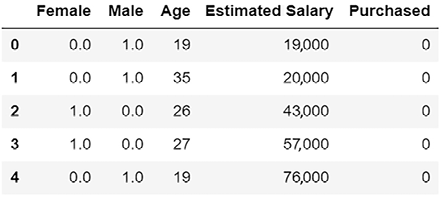
Figure 7.2: Add a caption here….

Notice that in order to convert a variable from a category variable into a continuous variable, one-hot encoding has converted Gender into two separate columns—Male and Female.

Let us look into how we can specify the features and labels.

Specifying the features and label

Let’s specify the features and labels. We will use y through out this book to represent the label and X to represent the feature set:

y=result['Purchased']
X=result.drop(columns=['Purchased'])

X represents the feature vector and contains all the input variables that we need to use to train the model.

Dividing the dataset into testing and training portions

Next, we will partition our dataset into two parts: 70% for training and 30% for testing. The rationale behind this particular division is that, as a rule of thumb in machine learning practice, we want a sizable portion of the dataset to train our model so that it can learn effectively from various examples. This is where the larger 70% comes into play. However, we also need to ensure that our model generalizes well to unseen data and doesn’t just memorize the training set. To evaluate this, we will set aside 30% of the data for testing. This data is not used during the training process and acts as a benchmark for gauging the trained model’s performance and its ability to make predictions on new, unseen data:

X_train, X_test, y_train, y_test = train_test_split(X, y,test_size = 0.25, random_state = 0)

This has created the following four data structures:

• X_train: A data structure containing the features of the training data
• X_test: A data structure containing the features of the training test
• y_train: A vector containing the values of the label in the training dataset
• y_test: A vector containing the values of the label in the testing dataset

Let us now apply feature normalization to the dataset.

Scaling the features

As we proceed with the preparation of our dataset for our machine learning model, an important step is feature normalization, also known as scaling. In many machine learning algorithms, scaling the variables to a uniform range, typically from 0 to 1, can enhance the model’s performance by ensuring that no individual feature can dominate others due to its scale.

This process can also help the algorithm converge more quickly to the solution. Now, let’s apply this transformation to our dataset for optimal results.

First, we initialize an instance of the StandardScaler class, which will be used to conduct the scaling operation:

# Feature Scaling
sc = StandardScaler()

Then, we use the fit_transform method. This transformation scales the features such that they have a mean of 0 and a standard deviation of 1, which is the essence of standard scaling. The transformed data is stored in the X_train_scaled variable:

X_train = sc.fit_transform(X_train)

Next, we will apply the transform method, which applies the same transformation (as in the prior code) to the test dataset X_test:

X_test = sc.transform(X_test)

After we scale the data, it is ready to be used as input to the different classifiers that we will present in the subsequent sections.

Evaluating the classifiers

Once the model is trained, we need to evaluate its performance. To do that, we will use the following process:

1. We will divide the labeling dataset into two parts—a training partition and a testing partition. We will use the testing partition to evaluate the trained model.
2. We will use the features of our testing partition to generate labels for each row. This is our set of predicted labels.
3. We will compare the set of predicted labels with the actual labels to evaluate the model.

Once we have both the set of actual labels and the predicted labels, a bunch of performance metrics can be used to evaluate the models.

The best metric for quantifying the model will depend on the requirements of the business problem that we want to solve, as well as the characteristics of the training dataset.

Let us now look at the confusion matrix.

Confusion matrices

A confusion matrix is used to summarize the results of the evaluation of a classifier. The confusion matrix for a binary classifier looks as follows:

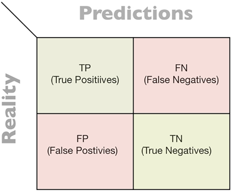
Figure 7.3: Confusion matrix

The classification can be divided into the following four categories:

• True Positives (TPs): The positive classifications that were correctly classified
• True Negatives (TNs): The negative classifications that were correctly classified
• False Positives (FPs): The positive classifications that were actually negative
• False Negatives (FNs): The negative classifications that were actually positive

Let’s see how we can use these four categories to create various performance metrics.

A confusion matrix provides a comprehensive snapshot of a model’s performance by detailing the number of correct and incorrect predictions. It enumerates TPs, TNs, FPs, and FNs. Among these, the correct classifications refer to the instances where our model correctly identified the class, i.e., TPs and TNs. The model’s accuracy, which signifies the proportion of these correct classifications (TPs and TNs) out of all the predictions made, can then be calculated directly from this confusion matrix. A confusion matrix gives you the number of correct classifications and misclassifications through a count of TPs, TNs, FPs, and FNs. The model accuracy is defined as the proportion of correct classifications among all predictions and can be easily seen from the confusion matrix as follows.

When we have an approximately equal number of positive and negative examples in our data – a situation known as balanced classes – the accuracy metric can provide a valuable measure of our model’s performance. In other words, accuracy is the ratio of correct predictions made by the model to the total number of predictions. For example, if our model correctly identifies 90 out of 100 test instances, whether they are positive or negative, its accuracy will be 90%. This metric can give us a general understanding of how well our model performs across both classes. If our data has balanced classes (i.e., the total number of positive examples is roughly equal to the number of negative examples), than the accuracy will give us a good insight into the quality of our trained model. Accuracy is the proportion of correction classifications among all predictions.

Mathematically:

Understanding recall and precision

While calculating accuracy, we do not differentiate between TPs and TNs. Evaluating a model through accuracy is straightforward, but when the data has imbalanced classes, it will not accurately quantify the quality of the trained model. When the data has imbalanced classes, two additional metrics will better quantify the quality of the trained model, recall and precision. We will use an example of a popular diamond mining process to explain the concepts of these two additional metrics.

For centuries, alluvial diamond mining has been one of the most popular ways of extracting diamonds from the sand of riverbeds all over the world. Erosion over thousands of years is known to wash diamonds from their primary deposits to riverbeds in different parts of the world. To mine diamonds, people have collected sand from the banks of rivers in a large open pit. After going though extensive washing, a large number of rocks are left in the pit.

A vast majority of these washed rocks are just ordinary stones. Identifying one of the rocks as a diamond is rare but a very important event. In our scenario, the owners of a mine are experimenting with the use of computer vision to identify which of the washed rocks are just ordinary rocks and which of the washed rocks are diamonds. They are using shape, color, and reflection to classify the washed rocks using computer vision.

In the context of this example:

Let us explain recall and precision while keeping this diamond extraction process from the mine in mind:

• Recall: This calculates the hit rate, which is the proportion of identified events of interest in a gigantic repository of events. In other words, this metric rates our ability to find or “hit” most of the events of interest and leaves as little as possible unidentified. In the context of identifying diamonds in a pit of a large number of washed stones, recall is about quantifying the success of the treasure hunt. For a certain pit filled up with washed stones, recall will be the ratio of the number of diamonds identified to the total number of diamonds in the pit:

  

  Let us assume there were 10 diamonds in the pit, each valued at $1,000. Our machine learning algorithm was able to identify nine of them. So, the recall will be 9/10 = 0.90.

  So, we are able to retrieve 90% of our treasure. In dollar cost, we were able to identify $9,000 of treasure out of a total value of $10,000.

• Precision: In precision, we only focus on the data points flagged by the trained model as positive and discard everything else. If we filter only the events flagged as positive by our trained model (i.e., TPs and FPs) and then calculate the accuracy, this is called precision.

  Now, let us investigate precision in the context of the diamond mining example. Let us consider a scenario where we want to use computer vision to identify diamonds among a pit of washed rocks and send them to customers.

  The process is supposed to be automated. The worst-case scenario is the algorithm misclassifying a stone as a diamond, resulting in the end customer receiving it in the mail and getting charged for it. So, it should be obvious that for this process to be feasible, precision should be high.

  For the diamond mining example:

  

Understanding the recall and precision trade-off

Making decisions with a classifier involves a two-step process. Firstly, the classifier generates a decision score ranging from 0 to 1. Then, it applies a decision threshold to determine the class for each data point. Data points scoring above the threshold are assigned a positive class, while those scoring below are assigned a negative class. The two steps can be explained as follows:

1. The classifier generates a decision score, which is a number from 0 to 1.
2. The classifier uses the value of a parameter, called a decision threshold, to allocate one of the two classes to the current datapoint. Any decision (score > decision) threshold is predicted to be positive, and any data point having a decision (score < decision) threshold is predicted to be negative.

Envision a scenario where you operate a diamond mine. Your task is to identify precious diamonds in a heap of ordinary rocks. To facilitate this process, you’ve developed a machine learning classifier. The classifier reviews each rock, assigns it a decision score ranging from 0 to 1, and finally, classifies the rock based on this score and a predefined decision threshold.

The decision score essentially represents the classifier’s confidence that a given rock is indeed a diamond, with rocks closer to 1 highly likely to be diamonds. The decision threshold, on the other hand, is a predefined cut-off point that decides the ultimate classification of a rock. Rocks scoring above the threshold are classified as diamonds (the positive class), while those scoring below are discarded as ordinary rocks (the negative class).

Now, imagine all the rocks are arranged in ascending order of their decision scores, as shown in Figure 7.4. The rocks on the far left have the lowest scores and are least likely to be diamonds, while those on the far right have the highest scores, making them most likely to be diamonds. In an ideal scenario, every rock to the right of the decision threshold would be a diamond, and every rock to the left would be an ordinary stone.

Consider a situation, as depicted in Figure 7.4, where the decision threshold is at the center. On the right side of the decision boundary, we find three actual diamonds (TPs) and one ordinary rock wrongly flagged as a diamond (FPs). On the left, we have two ordinary rocks correctly identified (TNs) and two diamonds wrongly classified as ordinary rocks (FNs).

Thus, on the left-hand side of the decision threshold, you will find two correct classifications and two misclassifications. They are 2TNs and 2FNs.

Let us calculate the recall and precision for Figure 7.4:

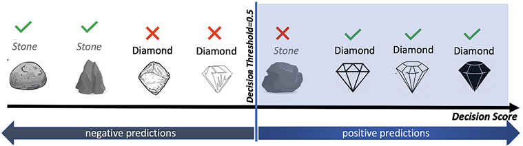
Figure 7.4: Precision/recall trade-off: rocks are ranked by their classifier score

Those that are above the decision threshold are considered diamonds.

Note that the higher the threshold, the higher the precision but the lower the recall.

Adjusting the decision threshold influences the trade-off between precision and recall. If we move the threshold to the right (as shown in Figure 7.5), we increase the criteria for a rock to be classified as a diamond, increasing precision but decreasing recall:

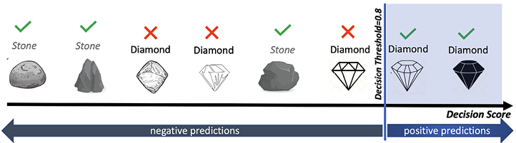
Figure 7.5: Precision/recall trade-off: rocks are ranked by their classifier score

Those that are above the decision threshold are considered diamonds. Note that the higher the threshold, the higher the precision but the lower the recall.

In Figure 7.6, we have decreased the decision threshold. In other words, we have decreased our criteria for a rock to be classified as a diamond. So, FNs (the treasure misses) will decrease, but FPs (the false signal) will increase as well. Thus, if we decrease the threshold (as shown in Figure 7.6), we loosen the criteria for diamond classification, increasing recall but decreasing precision:

Figure 7.6: Precision/recall trade-off: rocks are ranked by their classifier score

Those that are above the decision threshold are considered diamonds. Note that the higher the threshold, the higher the precision but the lower the recall.

So, playing with the value of the decision boundary is about managing the trade-off between recall and precision. We increase the decision boundary to get better precision and can expect more recall, and we lower the decision boundary to get better recall and can expect less precision.

Let us draw a graph between precision and recall to better understand the trade-off:

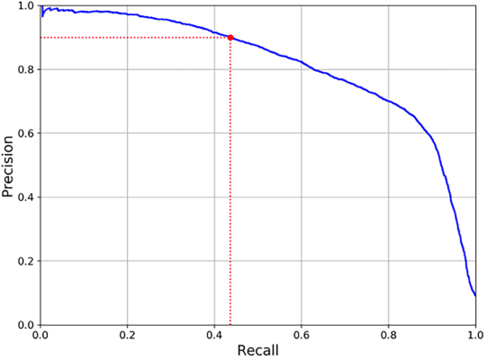
Figure 7.7: Precision vs. recall

What is the right choice for recall and precision?

Increasing recall is done by decreasing the criteria we use to identify a data point as positive. The precision is expected to decrease, but as shown in the figure above, it falls sharply at around 0.8. This is the point where we can choose the right value of recall and precision. In the above graph, if we choose 0.8 as the recall, the precision is 0.75. We can interpret it as being able to flag 80% of all the data points of interest. We flag these data points 75% accurately according to this level of precision. If there is no specific business requirement and it’s for a generic use case, this may be a reasonable compromise.

Another way to show the inherent trade-off between precision and recall is by using the Receiving Operating Curve (ROC). To do that, let us define two terms: True Positive Rate (TPR) and False Positive Rate (FPR).

Let us look into the ROC curve. To calculate the TPR and FPR, we need to look at the diamonds in the pit:

Note that:

• TPR is equal to the recall or hit rate.
• TNR can be thought of as the recall or hit rate of the negative event. It determines our success in correctly identifying the negative event. It is also called specificity.
• FPR = 1 – TNR = 1 - Specificity.

It should be obvious that TPR and FPR for these figures can be calculated as follows:

Note that TPR or recall will be increased by lowering our decision threshold. In an effort to get as many diamonds as possible from the mine, we will lower our criterion for a washed stone being classified as a diamond. The result is that more stones will be incorrectly classified as diamonds, increasing FPR.

Note that a good-quality classification algorithm should be able to provide the decision score for each of the rocks in the pit, which roughly matches the likelihood of a rock being a diamond. The output of such an algorithm is shown in Figure 7.8. Diamonds are supposed to be on the right side and stones are supposed to be on the left side. In the figure, as we have decreased the decision threshold from 0.8 to 0.2, we expect to have a much higher increase in TRP and then FPR. In fact, the steep increase in TRP with a slight increase in FPR is one of the best indications of the quality of a binary classifier, as the classification algorithm was able to generate decision scores that directly relate with the likelihood of a rock being a diamond. If the diamonds and stones are randomly located on the decision score axis, it is equally likely that lowering the decision threshold will flag stones or diamonds. This would be the worst possible binary classifier, also called a randomizer:

Figure 7.8: ROC curve

Understanding overfitting

If a machine learning model performs great in a development environment but degrades noticeably in a production environment, we say that the model is overfitted. This means the trained model too closely follows the training dataset. It is an indication there are too many details in the rules created by the model. The trade-off between model variance and bias best captures the idea.

When developing a machine learning model, we often make certain simplifying assumptions about the real-world phenomena that the model is supposed to capture. These assumptions are essential to make the modeling process manageable and less complex. However, the simplicity of these assumptions introduces a certain level of ‘bias’ in to our model.

Let’s break this down further. Bias is a term that quantifies how much, on average, our predictions deviate from true values. In simple terms, if we have high bias, it means our model’s predictions are far off from the actual values, which leads to a high error rate on our training data.

For instance, consider linear regression models. They assume a linear relationship between input features and output variables. However, this may not always be the case in real-world scenarios where relationships can be non-linear or more complex. This linear assumption, while simplifying our model, can lead to a high bias, as it may not fully capture the actual relationships between variables.

Now, let’s also talk about ‘variance.’ Variance, in the context of machine learning, refers to the amount by which our model’s predictions would change if we used a different training dataset. A model with high variance pays a lot of attention to training data and tends to learn from the noise and the details. As a result, it performs very well on training data but not so well on unseen or test data. This difference in performance is often referred to as overfitting.

We can visualize bias and variance using a bullseye diagram, as shown in Figure 7.9. Note that the center of the target is a model that perfectly predicts the correct values. Shots that are far away from the bullseye indicate high bias, while shots that are dispersed widely indicate high variance. In a perfect scenario, we would like a low bias and low variance, where all shots hit right in the bullseye. However, in real-world scenarios, there is a trade-off. Lowering bias increases variance, and lowering variance increases bias.

This is known as the bias-variance trade-off and is a fundamental aspect of machine learning model design:

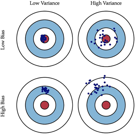
Figure 7.9: Graphical illustration of bias and variance

Balancing the right amount of generalization in a machine learning model is a delicate process. This balance, or sometimes imbalance, is described by the bias-variance trade-off. Generalization in machine learning refers to the model’s ability to adapt properly to new, unseen data, drawn from the same distribution as the one used for training. In other words, a well-generalized model can effectively apply learned rules from training data to new, unseen data. A more generalized model is achieved using simpler assumptions. These simpler assumptions result in more broad rules, which in turn make the model less sensitive to fluctuations in the training data. This means that the model will have low variance, as it doesn’t change much with different training sets.

However, there is a downside to this. Simpler assumptions mean the model might not fully capture all the complex relationships within the data. This results in a model that is consistently ‘off-target’ from the true output, leading to a higher bias.

So, in this sense, more generalization equates to lower variance but higher bias. This is the essence of the bias-variance trade-off: a model with too much generalization (high bias) might oversimplify the problem and miss important patterns, while a model with too little generalization (high variance) might overfit to the training data, capturing noise along with the signal.

Striking a balance between these two extremes is one of the central challenges in machine learning, and the ability to manage this trade-off can often make the difference between a good model and a great one. This trade-off between bias and variance is determined by the choice of algorithm, the characteristics of the data, and various hyperparameters. It is important to achieve the right compromise between bias and variance, based on the requirements of the specific problem you try to solve.

Let us now look into how we can specify different phases of a classifier.

Specifying the phases of classifiers

Once the labeled data is prepared, the development of the classifiers involves training, evaluation, and deployment. These three phases of implementing a classifier are shown in the Cross-Industry Standard Process for Data Mining (CRISP-DM) life cycle in the following diagram (the CRISP-DM life cycle was explained in more detail in Chapter 5, Graph Algorithms):

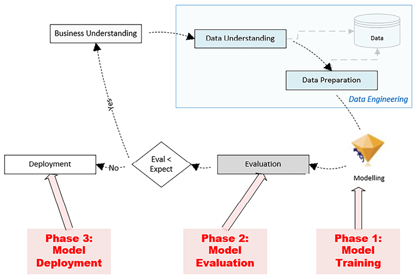
Figure 7.10: CRISP DM life cycle

When implementing a classifier model, there are several crucial phases to consider, starting with a thorough understanding of the business problem at hand. This involves identifying the data needed to solve this problem and understanding the real-world context of the data. After gathering the relevant labeled data, the next step is to split this dataset into two sections: a training set and a testing set. The training set, typically larger, is used to train the model to understand patterns and relationships within the data. The testing set, on the other hand, is used to evaluate the model’s performance on unseen data.

To ensure both sets are representative of the overall data distribution, we will use a random sampling technique. This way, we can reasonably expect that patterns in the entire dataset will be reflected in both the training and testing partitions.

Note that, as shown in Figure 7.10, there is first a training phase, where training data is used to train a model. Once the training phase is over, the trained model is evaluated using the testing data. Different performance matrices are used to quantify the performance of the trained model. Once the model is evaluated, we have the model deployment phase, where the trained model is deployed and used for inference to solve real-world problems by labeling unlabeled data.

Now, let’s look at some classification algorithms.

We will look at the following classification algorithms in the subsequent sections:

• The decision tree algorithm
• The XGBoost algorithm
• The Random Forest algorithm
• The logistic regression algorithm
• The SVM algorithm
• The Naive Bayes algorithm

Let’s start with the decision tree algorithm.

Decision tree classification algorithm

A decision tree is based on a recursive partitioning approach (divide and conquer), which generates a set of rules that can be used to predict a label. It starts with a root node and splits it into multiple branches. Internal nodes represent a test on a certain attribute, and the result of the test is represented by a branch to the next level. The decision tree ends in leaf nodes, which contain the decisions. The process stops when partitioning no longer improves the outcome.

Let us now look into the details of the decision tree algorithm.

Understanding the decision tree classification algorithm

The distinguishing feature of decision tree classification is the generation of a human-interpretable hierarchy of rules that is used to predict the label at runtime. This model’s transparency is a major advantage, as it allows us to understand the reasoning behind each prediction. This hierarchical structure is formed through a recursive algorithm, following a series of steps.

First, let’s illustrate this with a simplified example. Consider a decision tree model predicting whether a person will enjoy a specific movie. The topmost decision or ‘rule’ in the tree might be, ‘Is the movie a comedy or not?’ If the answer is yes, the tree branches to the next rule, like, ‘Does the movie star the person’s favorite actor?’ If no, it branches to another rule. Each decision point creates further subdivisions, forming a tree-like structure of rules, until we reach a final prediction.

With this process, a decision tree guides us through a series of understandable, logical steps to arrive at a prediction. This clarity is what sets decision tree classifiers apart from other machine learning models.

The algorithm is recursive in nature. Creating this hierarchy of rules involves the following steps:

1. Find the most important feature: Out of all of the features, the algorithm identifies the feature that best differentiates between the data points in the training dataset with respect to the label. The calculation is based on metrics such as information gain or Gini impurity.
2. Bifurcate: Using the most identified important feature, the algorithm creates a criterion that is used to divide the training dataset into two branches:
   • Data points that pass the criterion
   • Data points that fail the criterion
3. Check for leaf nodes: If any resultant branch mostly contains labels of one class, the branch is made final, resulting in a leaf node.
4. Check the stopping conditions and repeat: If the provided stopping conditions are not met, then the algorithm will go back to step 1 for the next iteration. Otherwise, the model is marked as trained, and each node of the resultant decision tree at the lowest level is labeled as a leaf node. The stopping condition can be as simple as defining the number of iterations, or a default stopping condition can be used, where the algorithm stops as soon it reaches a certain homogeneity level for each of the leaf nodes.

The decision tree algorithm can be explained by the following diagram:

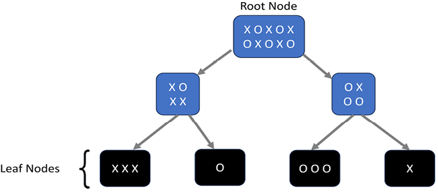
Figure 7.11: Decision Tree

In the preceding diagram, the root contains a bunch of circles and crosses. They just represent two different categories of a particular feature. The algorithm creates a criterion that tries to separate the circles from the crosses. At each level, the decision tree creates partitions of the data, which are expected to be more and more homogeneous from level 1 upward. A perfect classifier has leaf nodes that only contain circles or crosses. Training perfect classifiers is usually difficult due to the inherent unpredictability and noise in real-world datasets.

Note that the decision trees have key advantages that make them a preferred choice in many scenarios. The beauty of decision tree classifiers lies in their interpretability. Unlike many other models, they provide a clear and transparent set of ‘if-then’ rules, which makes the decision-making process understandable and auditable. This is particularly beneficial in fields like healthcare or finance, where comprehending the logic behind a prediction can be as important as the prediction itself.

Additionally, decision trees are less sensitive to the scale of the data and can handle a mix of categorical and numerical variables. This makes them a versatile tool in the face of diverse data types.

So, even though training a ‘perfect’ decision tree classifier might be difficult, the advantages they offer, including their simplicity, transparency, and flexibility, often outweigh this challenge.

We are going to use the decision tree classification algorithm for the classifiers challenge.

Now, let’s use the decision tree classification algorithm for the common problem that we previously defined to predict whether a customer ends up purchasing a product:

1. First, let’s instantiate the decision tree classification algorithm and train a model using the training portion of the data that we prepared for our classifiers:

   classifier = sklearn.tree.DecisionTreeClassifier(criterion = 'entropy', random_state = 100, max_depth=2)
   

   DecisionTreeClassifier(criterion = 'entropy', random_state = 100, max_depth=2)
   
2. Now, let’s use our trained model to predict the labels for the testing portion of our labeled data. Let’s generate a confusion matrix that can summarize the performance of our trained model:

   y_pred = classifier.predict(X_test)
   cm = metrics.confusion_matrix(y_test, y_pred)
   
3. This gives the following output:

   cm
   

   array([[64, 4],
          [2, 30]])
   
4. Now, let’s calculate the accuracy, recall, and precision values for the created classifier by using the decision tree classification algorithm:

   accuracy= metrics.accuracy_score(y_test,y_pred)
   recall = metrics.recall_score(y_test,y_pred)
   precision = metrics.precision_score(y_test,y_pred)
   print(accuracy,recall,precision)
   
5. Running the preceding code will produce the following output:

   0.94 0.9375 0.8823529411764706
   

The performance measures help us compare different training modeling techniques with each other.

Let us now look into the strengths and weaknesses of decision tree classifiers.

The strengths and weaknesses of decision tree classifiers

In this section, let’s look at the strengths and weaknesses of using the decision tree classification algorithm.

One of the most significant strengths of decision tree classifiers lies in their inherent transparency. The rules that govern their model formation are human-readable and interpretable, making them ideal for situations that demand a clear understanding of the decision-making process. This type of model, often referred to as a white-box model, is an essential component in scenarios where bias needs to be minimized and transparency maximized. This is particularly relevant in critical industries such as government and insurance, where accountability and traceability are paramount.

In addition, decision tree classifiers are well equipped to handle categorical variables. Their design is inherently suited to extracting information from discrete problem spaces, which makes them an excellent choice for datasets where most features fall into specific categories.

On the flip side, decision tree classifiers do exhibit certain limitations. Their biggest challenge is the tendency toward overfitting. When a decision tree delves too deep, it runs the risk of creating rules that capture an excessive amount of detail. This leads to models that overgeneralize from the training data and perform poorly on unseen data. Therefore, it’s critical to implement strategies such as pruning to prevent overfitting when using decision tree classifiers.

Another limitation of decision tree classifiers is their struggle with non-linear relationships. Their rules are predominantly linear, and as such, they may not capture the nuances of relationships that aren’t straight-line in nature. Therefore, while decision trees bring some impressive strengths to the table, their weaknesses warrant careful consideration when choosing the appropriate model for your data.

Use cases

Decision trees classifiers can be used in the following use cases to classify data:

• Mortgage applications: To train a binary classifier to determine whether an applicant is likely to default.
• Customer segmentation: To categorize customers into high-worth, medium-worth, and low-worth customers so that marketing strategies can be customized for each category.
• Medical diagnosis: To train a classifier that can categorize a benign or malignant growth.
• Treatment-effectiveness analysis: To train a classifier that can flag patients who have reacted positively to a particular treatment.
• Using a decision tree for feature selection: Another aspect worth discussing when examining decision tree classifiers is their feature selection capability. In the process of rule creation, decision trees tend to choose a subset of features from your dataset. This inherent trait of decision trees can be beneficial, especially when dealing with datasets that have a large number of features.

Why is this feature selection important, you might ask? In machine learning, dealing with numerous features can be a challenge. An excess of features can lead to models that are complex, harder to interpret, and may even result in worse performance due to the ‘curse of dimensionality.’

By automatically selecting a subset of the most important features, decision trees can simplify a model and focus on the most relevant predictors.

Notably, the feature selection process within decision trees isn’t confined to their own model development. The outcomes of this process can also serve as a form of preliminary feature selection for other machine learning models. This can provide an initial understanding of which features are most important and help streamline the development of other machine learning models.

Next, let us look into the ensemble methods.

Understanding the ensemble methods

In the domain of machine learning, an ensemble refers to a technique where multiple models, each with slight variations, are created and combined to form a composite or aggregate model. The variations could arise from using different model parameters, subsets of the data, or even different machine learning algorithms.

However, what does “slightly different” mean in this context? Here, each individual model in the ensemble is created to be unique, but not radically different. This can be achieved by tweaking the hyperparameters, training each model on a different subset of training data, or using diverse algorithms. The aim is to have each model capture different aspects or nuances of the data, which can help enhance the overall predictive power when they’re combined.

So, how are these models combined? The ensemble technique involves a process of decision-making known as aggregation, where the predictions from individual models are consolidated. This could be a simple average, a majority vote, or a more complex approach, depending on the specific ensemble technique used.

As for when and why ensemble methods are needed, they can be particularly useful when a single model isn’t sufficient to achieve a high level of accuracy. By combining multiple models, the ensemble can capture more complexity and often achieve better performance. This is because the ensemble can average out biases, reduce variance, and is less likely to overfit to the training data.

Finally, assessing the effectiveness of an ensemble is similar to evaluating a single model. Metrics such as accuracy, precision, recall, or F1-score can be used, depending on the nature of the problem. The key difference is that these metrics are applied to the aggregated predictions of the ensemble rather than the predictions of a single model.

Let’s look at some ensemble algorithms, starting with XGBoost.

Implementing gradient boosting with the XGBoost algorithm

XGBoost, introduced in 2014, is an ensemble classification algorithm that’s gained widespread popularity, primarily due to its foundation on the principles of gradient boosting. But what does gradient boosting entail? Essentially, it’s a machine learning technique that involves building many models sequentially, with each new model attempting to correct the errors made by the previous ones. This progression continues until a significant reduction in error rate is achieved, or a pre-defined number of models has been added.

In the context of XGBoost, it employs a collection of interrelated decision trees and optimizes their predictions using gradient descent, a popular optimization algorithm that aims to find the minimum of a function – in this case, the residual error. In simpler terms, gradient descent iteratively adjusts the model to minimize the difference between its predictions and the actual values.

The design of XGBoost makes it well suited for distributed computing environments. This compatibility extends to Apache Spark – a platform for large-scale data processing, and cloud computing platforms like Google Cloud and Amazon Web Services (AWS). These platforms provide the computational resources needed to efficiently run XGBoost, especially on larger datasets.

Now, we will walk through the process of implementing gradient boosting using the XGBoost algorithm. Our journey includes preparing the data, training the model, generating predictions, and evaluating the model’s performance. Firstly, data preparation is key to properly utilizing the XGBoost algorithm. Raw data often contains inconsistencies, missing values, or variable types that might not be suitable for the algorithm. Therefore, it’s imperative to preprocess and clean the data, normalizing numerical fields and encoding categorical ones as needed. Once our data is appropriately formatted, we can proceed with model training. An instance of the XGBClassifier has been created, which we’ll use to fit our model. Let us look at the steps:

1. This process is trained using the X_train and y_train data subsets, representing our features and labels respectively:

   from xgboost import XGBClassifier
   classifier = XGBClassifier()
   classifier.fit(X_train, y_train)
   

   XGBClassifier(base_score=None, booster=None, callbacks=None,
                 colsample_bylevel=None, colsample_bynode=None,
                 colsample_bytree=None, early_stopping_rounds=None,
                 enable_categorical=False, eval_metric=None, feature_types=None,
                 gamma=None, gpu_id=None, grow_policy=None, importance_type=None,
                 interaction_constraints=None, learning_rate=None, max_bin=None,
                 max_cat_threshold=None, max_cat_to_onehot=None,
                 max_delta_step=None, max_depth=None, max_leaves=None,
                 min_child_weight=None, missing=nan, monotone_constraints=None,
                 n_estimators=100, n_jobs=None, num_parallel_tree=None,
                 predictor=None, random_state=None, ...)
   
2. Then, we will generate predictions based on the newly trained model:

   y_pred = classifier.predict(X_test)
   cm = metrics.confusion_matrix(y_test, y_pred)
   
3. The produces the following output:

   cm
   

   array([[64, 4],
          [4, 28]])
   
4. Finally, we will quantify the performance of the model:

   accuracy = metrics.accuracy_score(y_test,y_pred)
   recall = metrics.recall_score(y_test,y_pred)
   precision = metrics.precision_score(y_test,y_pred)
   print(accuracy,recall,precision)
   
5. This gives us the following output:

   0.92 0.875 0.875
   

Now, let’s look at the Random Forest algorithm.

The Random Forest algorithm is an ensemble learning method that achieves its effectiveness by combining the outputs of numerous decision trees, thereby reducing both bias and variance. Here, let’s dive deeper into how it’s trained and how it generates predictions. In training, the Random Forest algorithm leverages a technique known as bagging, or bootstrap-aggregating. It generates N subsets from the training dataset, each created by randomly selecting some rows and columns from the input data. This selection process introduces randomness into the model, hence the name ‘Random Forest.’ Each subset of data is used to train an independent decision tree, resulting in a collection of trees denoted as C₁ through C_m. These trees can be of any type, but typically, they’re binary trees where each node splits the data based on a single feature.

In terms of predictions, the Random Forest model employs a democratic voting system. When a new instance of data is fed into the model for prediction, each decision tree in the forest generates its own label. The final prediction is determined by majority voting, meaning the label that received the most votes from all the trees becomes the overall prediction.

It is shown in Figure 7.12:

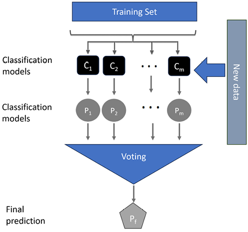
Figure 7.12: Random Forest

Note that in Figure 7.12, m trees are trained, which is represented by C₁ to C_m—that is, Trees = {C₁,..,C_m}.

Each of the trees generates a prediction, which is represented by a set:

Individual predictions = P= {P₁,..., P_m}

The final prediction is represented by Pf. It is determined by the majority of the individual predictions. The mode function can be used to find the majority decision (mode is the number that repeats most often and is in the majority). The individual prediction and the final prediction are linked, as follows:

Pf = mode (P)

This ensemble technique offers several benefits. Firstly, the randomness introduced into both data selection and decision tree construction reduces the risk of overfitting, increasing model robustness. Secondly, each tree in the forest operates independently, making Random Forest models highly parallelizable and, hence, suitable for large datasets. Lastly, Random Forest models are versatile, capable of handling both regression and classification tasks, and dealing effectively with missing or outlier data.

However, keep in mind that the effectiveness of a Random Forest model heavily depends on the number of trees it contains. Having too few might lead to a weak model, while too many could result in unnecessary computation. It’s important to fine-tune this parameter based on the specific needs of your application.

Differentiating the Random Forest algorithm from ensemble boosting

Random Forest and ensemble boosting represent two distinct approaches to ensemble learning, a powerful method in machine learning that combines multiple models to create more robust and accurate predictions.

In the Random Forest algorithm, each decision tree operates independently, uninfluenced by the performance or structure of the other trees in the forest. Each tree is built from a different subset of the data and uses a different subset of features for its decisions, adding to the overall diversity of the ensemble. The final output is determined by aggregating the predictions from all the trees, typically through a majority vote.

Ensemble boosting, on the other hand, employs a sequential process where each model is aware of the mistakes made by its predecessors. Boosting techniques generate a sequence of models where each successive model aims to correct the errors of the previous one. This is achieved by assigning higher weights to the misclassified instances in the training set for the next model in the sequence. The final prediction is a weighted sum of the predictions made by all models in the ensemble, effectively giving more influence to more accurate models.

In essence, while Random Forest leverages the power of independence and diversity, ensemble boosting focuses on correcting mistakes and improving from past errors. Each approach has its own strengths and can be more effective, depending on the nature and structure of the data being modeled.

Using the Random Forest algorithm for the classifiers challenge

Let’s instantiate the Random Forest algorithm and use it to train our model using the training data.

There are two key hyperparameters that we’ll look at here:

• n_estimators
• max_depth

The n_estimators hyperparameter determines the number of individual decision trees that are constructed within the ensemble. Essentially, it dictates the size of the ‘forest.’ A larger number of trees generally leads to more robust predictions, as it increases the diversity of decision paths and a model’s ability to generalize. However, it’s important to note that adding more trees also increases the computational complexity, and beyond a certain point, the improvements in accuracy may become negligible.

On the other hand, the max_depth hyperparameter specifies the maximum depth that each individual tree can reach. In the context of a decision tree, ‘depth’ refers to the longest path from the root node (the starting point at the top of the tree) to a leaf node (the final decision outputs at the bottom). By limiting the maximum depth, we essentially control the complexity of the learned structures, balancing the trade-off between underfitting and overfitting. A tree that’s too shallow may miss important decision rules, while a tree that’s too deep may overfit to the training data, capturing noise and outliers.

Fine-tuning these two hyperparameters plays a vital role in optimizing the performance of your decision-tree-based models, striking the right balance between predictive power and computational efficiency.

To train a classifier using the Random Forest algorithm, we will do the following:

classifier = RandomForestClassifier(n_estimators = 10, max_depth = 4,
criterion = 'entropy', random_state = 0)
classifier.fit(X_train, y_train)

RandomForestClassifier(n_estimators = 10, max_depth = 4,criterion = 'entropy', random_state = 0)

Once the Random Forest model is trained, let’s use it for predictions:

y_pred = classifier.predict(X_test)
cm = metrics.confusion_matrix(y_test, y_pred)
cm

Which gives the output as:

array ([[64, 4],
        [3, 29]])

Now, let’s quantify how good our model is:

accuracy= metrics.accuracy_score(y_test,y_pred)
recall = metrics.recall_score(y_test,y_pred)
precision = metrics.precision_score(y_test,y_pred)
print(accuracy,recall,precision)

We will observe the following output:

0.93 0.90625 0.8787878787878788

Note that Random Forest is a popular and versatile machine learning method that can be used for both classification and regression tasks. It is renowned for its simplicity, robustness, and flexibility, making it applicable across a broad range of contexts.

Next, let’s look into logistic regression.

Logistic regression

Logistic regression is a classification algorithm used for binary classification. It uses a logistic function to formulate the interaction between the input features and the label. It is one of the simplest classification techniques that is used to model a binary dependent variable.

Assumptions

Logistic regression assumes the following:

• The training dataset does not have a missing value.
• The label is a binary category variable.
• The label is ordinal—in other words, a categorical variable with ordered values.
• All features or input variables are independent of each other.

Establishing the relationship

For logistic regression, the predicted value is calculated as follows:

Let’s suppose that:

So now:

The preceding relationship can be graphically shown as follows:

Figure 7.13: Plotting the sigmoid function

Note that if z is large, (z) will equal 1. If z is very small or a large negative number, (z) will equal 0. Also, when z is 0, then (z)=0.5. Sigmoid is a natural function to use to represent probabilities, as it is strictly bounded between 0 and 1. By ‘natural,’ we mean it is well suited or particularly effective due to its inherent properties. In this case, the sigmoid function always outputs a value between 0 and 1, which aligns with the probability range. This makes it a great tool for modeling probabilities in logistic regression. The objective of training a logistic regression model is to find the correct values for w and j.

The loss and cost functions

The loss function defines how we want to quantify an error for a particular example in our training data. The cost function defines how we want to minimize an error in our entire training dataset. So, the loss function is used for one of the examples in the training dataset and the cost function is used for the overall cost that quantifies the overall deviation of the actual and predicted values. It is dependent on the choice of w and h.

The loss function used in logistic regression for a certain example i in the training set is as follows:

Loss (ý⁽ⁱ⁾, y⁽ⁱ⁾) = - (y⁽ⁱ⁾ log ý⁽ⁱ⁾ + (1-y⁽ⁱ⁾ ) log (1-ý⁽ⁱ⁾)

Note that when y⁽ⁱ⁾ = 1, Loss(ý⁽ⁱ⁾, y⁽ⁱ⁾) = - logý⁽ⁱ⁾. Minimizing the loss will result in a large value of ý⁽ⁱ⁾. Being a sigmoid function, the maximum value will be 1.

If y⁽ⁱ⁾ = 0, Loss (ý⁽ⁱ⁾, y⁽ⁱ⁾) = - log (1-ý⁽ⁱ⁾).

Minimizing the loss will result in ý⁽ⁱ⁾ being as small as possible, which is 0.

The cost function of logistic regression is as follows:

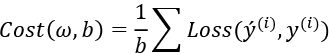
Let us now look into the details of logistic regression.

When to use logistic regression

Logistic regression works great for binary classifiers. To clarify, binary classification refers to the process of predicting one of two possible outcomes. For example, if we try to predict whether an email is spam or not, this is a binary classification problem because there are only two possible results – ‘spam’ or ‘not spam.’

However, there are certain limitations to logistic regression. Particularly, it may struggle when dealing with large datasets of subpar quality. For instance, consider a dataset filled with numerous missing values, outliers, or irrelevant features. The logistic regression model might find it difficult to produce accurate predictions under these circumstances.

Further, while logistic regression can handle linear relationships between features and the target variable effectively, it can fall short when dealing with complex, non-linear relationships. Picture a dataset where the relationship between the predictor variables and the target is not a straight line but a curve; a logistic regression model might struggle in such scenarios.

Despite these limitations, logistic regression can often serve as a solid starting point for classification tasks. It provides a benchmark performance that can be used to compare the effectiveness of more complex models. Even if it doesn’t deliver the highest accuracy, it does offer interpretability and simplicity, which can be valuable in certain contexts.

Using the logistic regression algorithm for the classifiers challenge

In this section, we will see how we can use the logistic regression algorithm for the classifiers challenge:

1. First, let’s instantiate a logistic regression model and train it using the training data:

   from sklearn.linear_model import LogisticRegression
   classifier = LogisticRegression(random_state = 0)
   classifier.fit(X_train, y_train)
   
2. Let’s predict the values of the test data and create a confusion matrix:

   y_pred = classifier.predict(X_test)
   cm = metrics.confusion_matrix(y_test, y_pred)
   cm
   
3. We get the following output upon running the preceding code:

   array ([[65, 3],
           [6, 26]])
   
4. Now, let’s look at the performance metrics:

   accuracy= metrics.accuracy_score(y_test,y_pred)
   recall = metrics.recall_score(y_test,y_pred)
   precision = metrics.precision_score(y_test,y_pred)
   print(accuracy,recall,precision)
   
5. We get the following output upon running the preceding code:

   0.91 0.8125 0.8996551724137931
   

Next, let’s look at SVMs.

The SVM algorithm

The SVM classifier is a robust tool in the machine learning arsenal, which functions by identifying an optimal decision boundary, or hyperplane, that distinctly segregates two classes. To further clarify, think of this ‘hyperplane’ as a line (in two dimensions), a surface (in three dimensions), or a manifold (in higher dimensions) that best separates the different classes in the feature space.

The key characteristic that sets SVMs apart is their optimization goal – it aims to maximize the margin, which is the distance between the decision boundary and the closest data points from either class, known as the ‘support vectors.’ In simpler terms, the SVM algorithm doesn’t just find a line to separate the classes; it also tries to find the line that’s as far away as possible from the closest points of each class, thereby maximizing the separating gap.

Consider a basic two-dimensional example where we try to separate circles from crosses. Our goal with SVMs is not just to find a line that divides these two types of shapes but also to find the line that maintains the greatest distance from the circles and crosses nearest to it.

SVMs can be extremely useful when dealing with high-dimensional data, complex domains, or when the classes are not easily separable by a simple straight line. They can perform exceptionally well where logistic regression may falter, for instance, in situations with non-linearly separable data.

The margin is defined as the distance between the separating hyperplane (the decision boundary) and the training samples that are closest to this hyperplane, called the support vectors. So, let’s start with a very basic example with only two dimensions, X₁ and X₂. We want a line to separate the circles from the crosses. This is shown in the following diagram:

Figure 7.14: SVM algorithm

We have drawn two lines, and both perfectly separate the crosses from the circles. However, there has to be an optimal line, or decision boundary, that gives us the best chance of correctly classifying most of the additional examples. A reasonable choice may be a line that is evenly spaced between these two classes to give a little bit of a buffer for each class, as shown here:

Figure 7.15: Concepts related to SVM

Moreover, unlike logistic regression, SVMs are better equipped to handle smaller, cleaner datasets, and they excel at capturing complex relationships without needing a large amount of data. However, the trade-off here is interpretability – while logistic regression provides easily understandable insights into the model’s decision-making process, SVMs, being inherently more complex, are not as straightforward to interpret.

Now, let’s see how we can use SVM to train a classifier for our challenge.

Using the SVM algorithm for the classifiers challenge

First, let’s instantiate the SVM classifier and then use the training portion of the labeled data to train it. The kernel hyperparameter determines the type of transformation that is applied to the input data in order to make it linearly separable:

from sklearn.svm import SVC
classifier = SVC(kernel = 'linear', random_state = 0)
classifier.fit(X_train, y_train)

1. Once trained, let’s generate some predictions and look at the confusion matrix:

   y_pred = classifier.predict(X_test)
   cm = metrics.confusion_matrix(y_test, y_pred)
   cm
   
2. Observe the following output:

   array ([[66, 2],
           [9, 23]])
   
3. Now, let’s look at the various performance metrics:

   accuracy= metrics.accuracy_score(y_test,y_pred)
   recall = metrics.recall_score(y_test,y_pred)
   precision = metrics.precision_score(y_test,y_pred)
   print(accuracy,recall,precision)
   

After running the preceding code, we get the following values as our output:

0.89 0.71875 0.92

Understanding the Naive Bayes algorithm

Based on probability theory, Naive Bayes is one of the simplest classification algorithms. If used properly, it can come up with accurate predictions. The Naive Bayes Algorithm is so-named for two reasons:

• It is based on a naive assumption that there is independence between the features and the input variable.
• It is based on Bayes’ theorem. Note that Bayes’ theorem is employed to calculate the probability of a particular class or outcome, given some observed features.

This algorithm tries to classify instances based on the probabilities of the preceding attributes/instances, assuming complete attribute independence.

There are three types of events:

• Independent events do not affect the probability of another event occurring (for example, receiving an email offering you free entry to a tech event and a re-organization occurring in your company).
• Dependent events affect the probability of another event occurring; that is, they are linked in some way (for example, the probability of you getting to a conference on time could be affected by an airline staff strike or flights that may not run on time).
• Mutually exclusive events cannot occur simultaneously (for example, the probability of rolling a three and a six on a single dice roll is 0—these two outcomes are mutually exclusive).

Bayes’ theorem

Bayes’ theorem is used to calculate the conditional probability between two independent events, A and B. The probability of events A and B happening is represented by P(A) and P(B). The conditional probability is represented by P(B|A), which is the conditional probability that event B will happen given that event A has occurred:

When it comes to applying Naive Bayes, the algorithm is particularly effective in scenarios where the dimensionality of the inputs (number of features) is high. This makes it well suited for text classification tasks such as spam detection or sentiment analysis.

It can handle both continuous and discrete data, and it’s computationally efficient, making it useful for real-time predictions. Naive Bayes is also a good choice when you have limited computational resources and need a quick and easy implementation, but it’s worth noting that its “naive” assumption of feature independence can be a limitation in some cases.

Calculating probabilities

Naive Bayes is based on probability fundamentals. The probability of a single event occurring (the observational probability) is calculated by taking the number of times the event occurred and dividing it by the total number of processes that could have led to that event. For example, a call center receives over 100 support calls per day, which is 50 times over the course of a month. You want to know the probability that a call is responded to in under three minutes, based on the previous amount of time in which it was responded to. If the call center manages to match this time record on 27 occasions, then the observational probability of 100 calls being answered in under three minutes is as follows:

P(100 support calls in under 3 mins) = (27 / 50) = 0.54 (54%)

One hundred calls can be responded to in under three minutes in about half the time, based on the records of the 50 times it occurred in the past.

Now, let us look into the multiplication rules for AND events.

Multiplication rules for AND events

To calculate the probability of two or more events occurring simultaneously, consider whether events are independent or dependent. If they are independent, the simple multiplication rule is used:

P(outcome 1 AND outcome 2) = P(outcome 1) * P(outcome 2)

For example, to calculate the probability of receiving an email with free entry to a tech event and re-organization occurring in your workplace, this simple multiplication rule would be used. The two events are independent, as the occurrence of one does not affect the chance of the other occurring.

If receiving the tech event email has a probability of 31% and the probability of staff re-organization is 82%, then the probability of both occurring is calculated as follows:

P(email AND re-organization) = P(email) * P(re-organization) = (0.31) * (0.82) = 0.2542 (25%)

The general multiplication rule

If two or more events are dependent, the general multiplication rule is used. This formula is actually valid in both cases of independent and dependent events:

P(outcome 1 AND outcome 2)=P(outcome 1)*P(outcome 2 | outcome 1)

Note that P(outcome 2 | outcome 1) refers to the conditional probability of outcome 2 occurring given that outcome 1 has already occurred. The formula incorporates the dependence between the events. If the events are independent, then the conditional probability is irrelevant as one outcome does not influence the chance of the other occurring, and P(outcome 2 | outcome 1) is simply P(outcome 2). Note that the formula in this case just becomes the simple multiplication rule.

Let’s illustrate this with a simple example. Suppose you’re drawing two cards from a deck, and you want to know the probability of drawing an ace first and then a king. The first event (drawing an ace) modifies the conditions for the second event (drawing a king) since we’re not replacing the ace in the deck. According to the general multiplication rule, we can calculate this as P(ace) * P(king | ace), where P(king | ace) is the probability of drawing a King given that we’ve already drawn an ace.

Addition rules for OR events

When calculating the probability of either one event or the other occurring (mutually exclusive), the following simple addition rule is used:

P(outcome 1 OR outcome 2) = P(outcome 1) + P(outcome 2)

For example, what is the probability of rolling a 6 or a 3? To answer this question, first, note that both outcomes cannot occur simultaneously. The probability of rolling a 6 is (1 / 6) and the same can be said for rolling a 3:

P(6 OR 3) = (1 / 6) + (1 / 6) = 0.33 (33%)

If the events are not mutually exclusive and can occur simultaneously, use the following general addition formula, which is always valid in both cases of mutual exclusiveness and non-mutual exclusiveness:

P(outcome 1 OR outcome 2) = P(outcome 1) + P(outcome 2) P(outcome 1 AND outcome 2)

Using the Naive Bayes algorithm for the classifiers challenge

Now, let’s use the Naive Bayes algorithm to solve the classifiers challenge:

1. First, we will import the GaussianNB() function and use it to train the model:

   # Fitting Decision Tree Classification to the Training set
   from sklearn.naive_bayes import GaussianNB
   classifier = GaussianNB()
   classifier.fit(X_train, y_train)
   

   GaussianNB()
   
2. Now, let’s use the trained model to predict the results. We will use it to predict the labels for our test partition, which is X_test:

   # Predicting the Test set results
   y_pred = classifier.predict(X_test)
   cm = metrics.confusion_matrix(y_test, y_pred)
   
3. Now, let’s print the confusion matrix:

   cm
   

   array([[66, 2],
   [6, 26]])
   
4. Now, let’s print the performance matrices to quantify the quality of our trained model:

   accuracy= metrics.accuracy_score(y_test,y_pred)
   recall = metrics.recall_score(y_test,y_pred)
   precision = metrics.precision_score(y_test,y_pred)
   print(accuracy,recall,precision)
   

Which gives the output as:

0.92 0.8125 0.9285714285714286

For classification algorithms, the winner is...

Let’s take a moment to compare the performance metrics of the various algorithms we’ve discussed. However, keep in mind that these metrics are highly dependent on the data we’ve used in these examples, and they can significantly vary for different datasets.

The performance of a model can be influenced by factors such as the nature of the data, the quality of the data, and how well the assumptions of the model align with the data.

Here’s a summary of our observations:

From the table above, the decision tree classifier exhibits the highest performance in terms of both accuracy and recall in this particular context. For precision, we see a tie between the SVM and Naive Bayes algorithms.

However, remember that these results are data-dependent. For instance, SVM might excel in scenarios where data is linearly separable or can be made so through kernel transformations. Naive Bayes, on the other hand, performs well when the features are independent. Decision trees and Random Forests might be preferred when we have complex non-linear relationships. Logistic regression is a solid choice for binary classification tasks and can serve as a good benchmark model. Lastly, XGBoost, being an ensemble technique, is powerful when dealing with a wide range of data types and often leads in terms of model performance across various tasks.

So, it’s critical to understand your data and the requirements of your task before choosing a model. These results are merely a starting point, and deeper exploration and validation should be performed for each specific use case.

Understanding regression algorithms

A supervised machine learning model uses one of the regression algorithms if the label is a continuous variable. In this case, the machine learning model is called a regressor.

To provide a more concrete understanding, let’s take a couple of examples. Suppose we want to predict the temperature for the next week based on historical data, or we aim to forecast sales for a retail store in the coming months.

Both temperatures and sales figures are continuous variables, which means they can take on any value within a specified range, as opposed to categorical variables, which have a fixed number of distinct categories. In such scenarios, we would use a regressor rather than a classifier.

In this section, we will present various algorithms that can be used to train a supervised machine learning regression model—or, put simply, a regressor. Before we go into the details of the algorithms, let’s first create a challenge for these algorithms to test their performance, abilities, and effectiveness.

Presenting the regressors challenge

Similar to the approach that we used with the classification algorithms, we will first present a problem to be solved as a challenge for all regression algorithms. We will call this common problem the regressors challenge. Then, we will use three different regression algorithms to address the challenge. This approach of using a common challenge for different regression algorithms has two benefits:

• We can prepare the data once and use the prepared data on all three regression algorithms.
• We can compare the performance of three regression algorithms in a meaningful way, as we will use them to solve the same problem.

Let’s look at the problem statement of the challenge.

The problem statement of the regressors challenge

Predicting the mileage of different vehicles is important these days. An efficient vehicle is good for the environment and is also cost-effective. The mileage can be estimated from the power of the engine and the characteristics of the vehicle. Let’s create a challenge for regressors to train a model that can predict the Miles per Gallon (MPG) of a vehicle based on its characteristics.

Let’s look at the historical dataset that we will use to train the regressors.

Exploring the historical dataset

The following are the features of the historical dataset data that we have:

The label for this problem is a continuous variable, MPG, that specifies the MPG for each of the vehicles.

Let’s first design the data processing pipeline for this problem.

Feature engineering using a data processing pipeline

Let’s see how we can design a reusable processing pipeline to address the regressors challenge. As mentioned, we will prepare the data once and then use it in all the regression algorithms. Let’s follow these steps:

1. We will start by importing the dataset, as follows:

   dataset = pd.read_csv('https://storage.googleapis.com/neurals/data/data/auto.csv')
   
2. Let’s now preview the dataset:

   dataset.head(5)
   
3. This is how the dataset will look:

Figure 7.16: Please add a caption here

4. Now, let’s proceed on to feature selection. Let’s drop the NAME column, as it is only an identifier that is needed for cars. Columns that are used to identify the rows in our dataset are not relevant to training the model. Let’s drop this column.
5. Let’s convert all of the input variables and impute all the null values:

   dataset=dataset.drop(columns=['NAME'])
   dataset.head(5)
   dataset= dataset.apply(pd.to_numeric, errors='coerce')
   dataset.fillna(0, inplace=True)
   

   Imputation improves the quality of the data and prepares it to be used to train the model. Now, let’s see the final step.

6. Let’s divide the data into testing and training partitions:

   y=dataset['MPG']
   X=dataset.drop(columns=['MPG'])
   # Splitting the dataset into the Training set and Test set
   from sklearn.model_selection import train_test_split
   from sklearn.cross_validation import train_test_split
   X_train, X_test, y_train, y_test = train_test_split(X, y, test_size = 0.25, random_state = 0)
   

This has created the following four data structures:

• X_train: A data structure containing the features of the training data
• X_test: A data structure containing the features of the training test
• y_train: A vector containing the values of the label in the training dataset
• y_test: A vector containing the values of the label in the testing dataset

Now, let’s use the prepared data on three different regressors so that we can compare their performance.

Linear regression

Among the assortment of supervised machine learning algorithms, linear regression is often seen as the most straightforward to grasp. Initially, we will explore simple linear regression and then gradually broaden our discussion to encompass multiple linear regression.

It’s important to note, however, that while linear regression is accessible and easy to implement, it is not always the ‘best’ choice in every circumstance. Each machine learning algorithm, including the ones we’ve discussed so far, comes with its unique strengths and limitations, and their effectiveness varies depending on the type and structure of the data at hand.

For instance, decision trees and Random Forests are excellent at handling categorical data and capturing complex non-linear relationships. SVMs can work well with high-dimensional data and are robust to outliers, while logistic regression is particularly effective for binary classification problems.

On the other hand, linear regression models are well suited to predicting continuous outcomes and can provide interpretability, which can be valuable in understanding the impact of individual features.

Simple linear regression

At its most basic level, linear regression establishes a relationship between two variables, usually represented as a single independent variable and a single dependent variable. Linear regression is a technique that enables us to study how changes in the dependent variable (plotted on the y-axis) are influenced by changes in the independent variable (plotted on the x-axis). It can be represented as follows:

This formula can be explained as follows:

• y is the dependent variable.
• X is the independent variable.
• is the slope that indicates how much the line rises for each increase in X.
• α is the intercept that indicates the value of y when X = 0.

Linear regression operates under these assumptions:

• Linearity: The relationship between independent and dependent variables is linear.
• Independence: The observations are independent of each other.
• No multicollinearity: The independent variables are not too highly correlated with each other.

Some examples of relationships between a single continuous dependent variable and a single continuous independent variable are as follows:

• A person’s weight and their calorie intake
• The price of a house and its area in square feet in a particular neighborhood
• The humidity in the air and the likelihood of rain

For linear regression, both the input (independent) variable and the target (dependent) variable must be numeric. The best relationship is found by minimizing the sum of the squares of the vertical distances of each point, from a line drawn through all the points. It is assumed that the relationship is linear between the predictor variable and the label. For example, the more money invested in research and development, the higher the sales.

Let’s look at a specific example. Let’s try to formulate the relationship between marketing expenditures and sales for a particular product. They are found to be directly relational to each other. The marketing expenditures and sales are drawn on a two-dimensional graph and are shown as blue diamonds. The relationship can best be approximated by drawing a straight line, as shown in the following graph:

Figure 7.17: Linear regression

Once the linear line is drawn, we can see the mathematical relationship between marketing expenditure and sales.

Evaluating the regressors

The linear line that we drew is an approximation of the relationship between the dependent and independent variables. Even the best line will have some deviation from the actual values, as shown here:

Figure 7.18: Evaluating regressors

A typical way of quantifying the performance of linear regression models is by using Root Mean Square Error (RMSE). This calculates the standard deviation of the errors made by the trained model mathematically. For example, in the training dataset, the loss function is calculated as follows:

Loss (ý⁽ⁱ⁾, y⁽ⁱ⁾) = 1/2(ý⁽ⁱ⁾- y⁽ⁱ⁾)2

This leads to the following cost function, which minimizes the loss of all of the examples in the training set:

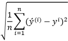
Let’s try to interpret RMSE. If RMSE is $50 for our example model that predicts the price of a product, this means that around 68.2% of the predictions will fall within $50 of the true value (that is, ). It also means that 95% of the predictions will fall within $100 (that is, ) of the actual value. Finally, 99.7% of the predictions will fall within $150 of the actual value.

Let us look into multiple regression.

Multiple regression

The fact is that most real-world analyses have more than one independent variable. Multiple regression is an extension of simple linear regression. The key difference is that there are additional beta coefficients for the additional predictor variables. When training a model, the goal is to find the beta coefficients that minimize the errors of the linear equation. Let’s try to mathematically formulate the relationship between the dependent variable and the set of independent variables (features).

For instance, in the housing market, the price of a house (the dependent variable) could depend on numerous factors such as its size, location, age, and more (the independent variables).

Similar to a simple linear equation, the dependent variable, y, is quantified as the sum of an intercept term, plus the product of the coefficients multiplied by the x value for each of the i features:

The error is represented by and indicates that the predictions are not perfect.

The coefficients allow each feature to have a separate estimated effect on the value of y because y changes by an amount of for each unit increase in x_i. Moreover, the intercept () indicates the expected value of y when the independent variables are all 0.

Note that all the variables in the preceding equation can be represented by a bunch of vectors. The target and predictor variables are now vectors with a row, and the regression coefficients, , and errors, , are also vectors.

Next, let us look into how we can use linear regression for the regressors challenge.

Using the linear regression algorithm for the regressors challenge

Now, let’s train the model using the training portion of the dataset. Note that we will use the same data and data engineering logic that we discussed earlier:

1. Let’s start by importing the linear regression package:

   from sklearn.linear_model import LinearRegression
   
2. Then, let’s instantiate the linear regression model and train it using the training dataset:

   regressor = LinearRegression()
   regressor.fit(X_train, y_train)
   

   LinearRegression()
   
3. Now, let’s predict the results using the test portion of the dataset:

   y_pred = regressor.predict(X_test)
   from sklearn.metrics import mean_squared_error
   sqrt(mean_squared_error(y_test, y_pred))
   
4. The output generated by running the preceding code will generate the following:

   19.02827669300187
   

As discussed in the preceding section, RMSE is the standard deviation of the error. It indicates that 68.2% of predictions will fall within 4.36 of the value of the label.

Let us look into when we can use linear regression.

When is linear regression used?

Linear regression is used to solve many real-world problems, including the following:

• Sales forecasting
• Predicting optimum product prices
• Quantifying the causal relationship between an event and the response, such as in clinical drug trials, engineering safety tests, or marketing research
• Identifying patterns that can be used to forecast future behavior, given known criteria—for example, predicting insurance claims, natural disaster damage, election results, and crime rates

Let us next look into the weaknesses of linear regression.

The weaknesses of linear regression

The weaknesses of linear regression are as follows:

• It only works with numerical features.
• Categorical data needs to be pre-processed.
• It does not cope well with missing data.
• It makes assumptions about the data.

The regression tree algorithm

Similar to classification trees used for categorical outcomes, regression trees are another subset of decision trees, but they are employed when the target, or label, is a continuous variable instead of categorical. This distinction impacts how the tree algorithm processes and learns from the data.

In the case of classification trees, the algorithm tries to identify the categories that the data points belong to. However, with regression trees, the goal is to predict a specific, continuous value. This might be something like the price of a house, a company’s future stock price, or the likely temperature tomorrow.

These variations between classification and regression trees also lead to differences in the algorithms used. In a classification tree, we typically use metrics such as Gini impurity or entropy to find the best split. In contrast, regression trees utilize measures like Mean Squared Error (MSE) to minimize the distance between the actual and predicted continuous values.

Using the regression tree algorithm for the regressors challenge

In this section, we will see how a regression tree algorithm can be used for the regressors challenge:

1. First, we train the model using a regression tree algorithm:

   from sklearn.tree import DecisionTreeRegressor
   regressor = DecisionTreeRegressor(max_depth=3)
   regressor.fit(X_train, y_train)
   

   DecisionTreeRegressor(max_depth=3)
   
2. Once the regression tree model is trained, we use the trained model to predict the values:

   y_pred = regressor.predict(X_test)
   
3. Then, we calculate RMSE to quantify the performance of the model:

   from sklearn.metrics import mean_squared_error
   from math import sqrt
   sqrt(mean_squared_error(y_test, y_pred))
   

We get the following output:

4.464255966462035

The gradient boost regression algorithm

Now, let’s shift our focus to the gradient boosting regression algorithm, which uses an ensemble of decision trees to formulate underlying patterns within a dataset.

At its core, gradient boosting regression operates by creating a ‘team’ of decision trees, where each member progressively learns from the mistakes of its predecessors. In essence, each subsequent decision tree in the sequence attempts to correct the prediction errors made by the tree before it, leading to an ‘ensemble’ that makes a final prediction based on the collective wisdom of all the individual trees. What makes this algorithm truly unique is its capability to handle a broad spectrum of data and its resistance to overfitting. This versatility allows it to perform admirably across diverse datasets and problem scenarios.

Using the gradient boost regression algorithm for the regressors challenge

In this section, we will see how we can use the gradient boost regression algorithm for the regressors challenge, predicting a car’s MPG rating, which is a continuous variable and, therefore, a classic regression problem. Remember that our independent variables include features like ‘CYLINDERS,’ ‘DISPLACEMENT,’ ‘HORSEPOWER,’ ‘WEIGHT,’ and ‘ACCELERATION.’

Looking closely, MPG is not as straightforward as it may seem, considering the multifaceted relationships between the influencing factors. For example, while cars with higher displacement typically consume more fuel, leading to a lower MPG, this relationship could be offset by factors like weight and horsepower. It’s these nuanced interactions that may elude simpler models like linear regression or a single decision tree.

This is where the gradient boosting regression algorithm may be useful. By building an ensemble of decision trees, each learning from the errors of its predecessor, the model will aim to discern these complex patterns in the data. Each tree contributes its understanding of the data, refining the predictions to be more accurate and reliable.

For example, one decision tree might learn that cars with larger ‘DISPLACEMENT' values tend to have lower MPG. The next tree might then pick up on the subtlety that lighter cars (‘WEIGHT') with the same ‘DISPLACEMENT' can sometimes achieve higher MPG. Through this iterative learning process, the model unveils the intricate layers of relationships between the variables:

1. The first step in our Python script is to import the necessary library:

   from sklearn import ensemble
   
2. Here, we import the ensemble module from the sklearn library:

   params = {'n_estimators': 500, 'max_depth': 4,          'min_samples_split': 2, 'learning_rate': 0.01,          'loss': 'squared_error'}
   regressor = ensemble.GradientBoostingRegressor(**params)
   regressor.fit(X_train, y_train)
   

   GradientBoostingRegressor(learning_rate=0.01, max_depth=4, n_estimators=500)
   

   y_pred = regressor.predict(X_test)
   
3. Finally, we calculate RMSE to quantify the performance of the model:

   from sklearn.metrics import mean_squared_error
   from math import sqrt
   sqrt(mean_squared_error(y_test, y_pred))
   
4. Running this will give us the output value, as follows:

   4.039759805419003
   

For regression algorithms, the winner is...

Let’s look at the performance of the three regression algorithms that we used on the same data and exactly the same use case:

Looking at the performance of all the regression algorithms, it is obvious that the performance of gradient boost regression is the best, as it has the lowest RMSE. This is followed by linear regression. The regression tree algorithm performed the worst for this problem.

Practical example – how to predict the weather

Now, we’ll transition from theory to application, employing the concepts we’ve discussed in this chapter to predict tomorrow’s rainfall, based on a year’s worth of weather data from a specific city. This real-world scenario aims to reinforce the principles of supervised learning.

There are numerous algorithms capable of this task, but selecting the most suitable one hinges on the specific characteristics of our problem and data. Each algorithm has unique advantages and excels in specific contexts. For example, while linear regression can be ideal when there’s a discernible numerical correlation, decision trees might be more effective when dealing with categorical variables or non-linear relationships.

For this prediction challenge, we have chosen logistic regression. This choice is driven by the binary nature of our prediction target (i.e., will it rain tomorrow or not?), a situation where Logistic Regression often excels. This algorithm provides a probability score between 0 and 1, allowing us to make clear yes-or-no predictions, ideal for our rainfall forecast scenario.

Remember, this practical example differs from previous ones. It’s crafted to help you grasp how we select and apply a particular algorithm to specific real-world problems, offering a deeper understanding of the thought process behind algorithm selection.

The data available to train this model is in the CSV file called weather.csv:

1. Let’s import the data as a pandas DataFrame:

   import numpy as np
   import pandas as pd
   df = pd.read_csv("weather.csv")
   
2. Let’s look at the columns of the DataFrame:

   df.columns
   

   Index(['Date', 'MinTemp', 'MaxTemp', 'Rainfall', 
          'Evaporation', 'Sunshine', 'WindGustDir', 
          'WindGustSpeed', 'WindDir9am', 'WindDir3pm', 
          'WindSpeed9am', 'WindSpeed3pm', 'Humidity9am', 
          'Humidity3pm', 'Pressure9am', 'Pressure3pm', 
          'Cloud9am', 'Cloud3pm', 'Temp9am', 'Temp3pm', 
          'RainToday', 'RISK_MM', 'RainTomorrow'],
         dtype='object')
   
3. Now, let’s look at the header of the first 13 columns of the weather.csv data that show the typical weather of a city:

   df.iloc[:,0:12].head()
   

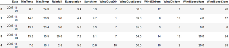
Figure 7.19: Data showing typical weather of a city

4. Now, let’s look at the last 10 columns of the weather.csv data:

   df.iloc[:,12:25].head()
   

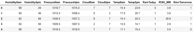
Figure 7.20: Last 10 columns of the weather.csv data

5. Let’s use x to represent the input features. We will drop the Date field for the feature list, as it is not useful in the context of predictions. We will also drop the RainTomorrow label:

   x = df.drop(['Date','RainTomorrow'],axis=1)
   
6. Let’s use y to represent the label:

   y = df['RainTomorrow']
   
7. Now, let’s divide the data into train_test_split:

   from sklearn.model_selection import train_test_split
   train_x , train_y ,test_x , test_y = train_test_split(x,y,
   test_size = 0.2,random_state = 2)
   
8. As the label is a binary variable, we will train a classifier. So, logistic regression will be a good choice here. First, let’s instantiate the logistic regression model:

   model = LogisticRegression()
   
9. Now, we can use train_x and test_x to train the model:

   model.fit(train_x , test_x)
   
10. Once the model is trained, let’s use it for predictions:

    predict = model.predict(train_y)
    
11. Now, let’s find the accuracy of our trained model:

    predict = model.predict(train_y)
    from sklearn.metrics import accuracy_score
    accuracy_score(predict , test_y)
    

    0.9696969696969697
    

Now, this binary classifier can be used to predict whether it will rain tomorrow.

Summary

Wrapping up, this chapter served as a comprehensive expedition into the multifaceted landscape of supervised machine learning. We spotlighted the primary components of classification and regression algorithms, dissecting their mechanics and applications.

The chapter demonstrated a broad spectrum of algorithms through practical examples, providing an opportunity to understand the functionality of these tools in real-world contexts. This journey underscored the adaptability of supervised learning techniques and their ability to tackle varied problems.

By juxtaposing the performance of different algorithms, we emphasized the crucial role of context when selecting an optimal machine learning strategy. Factors such as data size, feature complexity, and prediction requirements play significant roles in this selection process.

As we transition to the upcoming chapters, the knowledge gleaned from this exploration serves as a robust foundation. This understanding of how to apply supervised learning techniques in practical scenarios is a critical skill set in the vast realm of machine learning. Keep these insights at your fingertips as we journey further into the compelling world of AI, preparing for an even deeper dive into the complex universe of neural networks.

Learn more on Discord

To join the Discord community for this book – where you can share feedback, ask questions to the author, and learn about new releases – follow the QR code below:

https://packt.link/WHLel